Discovering a motif discovering appproach
LCG_BEII 2019
Jacques van Helden
2019-02-09
Goal of the exercise
The goal of this exercise is to get an intuition of a motif discovery approach relying on the detection of over-represented oligonucleotides.
Our approach will be pragmatic.
We retrieved the upstream non-coding sequences of the genes involved in methionine biosynthesis and sulfur assimilation, and counted the occurrences of each hexanucleotide.
We also computed
- the relative frequencies (occurrences of each oligo / sum of all oligo occurrences) in the sequence of interest (the promoters of methionine-associated genes)
- the relative frequencies of ach hexanucleotide in the whole set of yeast promoters.
We would like to know if some 6nt are over-reprsented in promoters of methionine-associated genes relative to the occurrences that would be expected from a random selection of yeast promoters.
Create a workspace for this practical
- In your home directory, create a work directory for this practical (for example
~/LCG_BEII/practical_motif_discovery/).
rmdDir <- getwd() # Path of this Rmd fiile

workdir <- "~/LCG_BEII/practical_motif_discovery"
dir.create(workdir, showWarnings = FALSE, recursive = TRUE)
setwd(workdir)
Loading the data table
- Download the oligonucleotide count table. Scerevisiae_MET-genes_oligos-6nt-2str-noov_occ-freq.tsv
oligo.url <- "http://jvanheld.github.io/LCG_BEII/practicals/motif_discovery/data/Scerevisiae_MET-genes_oligos-6nt-2str-noov_occ-freq.tsv"
oligo.file <- basename(oligo.url) ## Suppress the URL path and keep only the file name for local storage
download.file(oligo.url, destfile = oligo.file)
In R, open a new script or R markdown file.
Load the data table, print the 5 top rows and the 5 bottom rows.
oligo.table <- read.delim(oligo.file, header = 1, row.names = 1)
# View(oligo.table)

head(oligo.table, n = 5)
obs_freq exp_freq occ exp_occ
aaaaaa|tttttt 0.004592808 0.004896299 41 43.71
aaaaac|gttttt 0.001120197 0.001998518 10 17.84
aaaaag|cttttt 0.003696651 0.003604251 33 32.18
aaaaat|attttt 0.004032710 0.004160627 36 37.14
aaaaca|tgtttt 0.001344237 0.001932479 12 17.25tail(oligo.table, n = 5) obs_freq exp_freq occ exp_occ
ttccaa|ttggaa 0.0008961577 0.0008428396 8 7.52
ttcgaa|ttcgaa 0.0001120197 0.0003224542 1 2.88
ttgaaa|tttcaa 0.0019043352 0.0019087053 17 17.04
ttgcaa|ttgcaa 0.0001120197 0.0004030214 1 3.60
tttaaa|tttaaa 0.0005600986 0.0009379354 5 8.37Exploring observed and expected counts
- Draw an histogram of the observed occurrences and evaluate the spread of counts.
x <- oligo.table$occ
range(x)
[1] 0 45max.x <- max(x)
hist(x, breaks = 0:max.x, col = "palegreen",
xlab = "Observed occurrences",
ylab = "Nb of oligos",
las = 1,
main = "Distribution of oligonucelotide occurrences")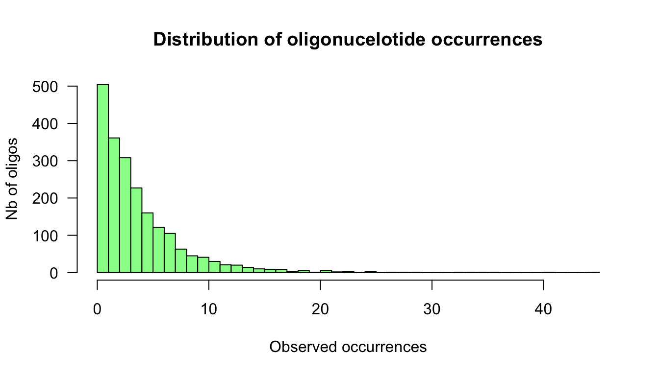
- Draw a scatter plot comparing the observed and expected occurrences for each hexanucleotide.
exp.occ <- oligo.table$exp_occ

plot(exp.occ, x, col = "grey", las = 1,
     xlab = "Expected occurrences",
     ylab = "Observed occurrences",
     main = "Observed vs expected occurrences")
grid()
abline(a = 0, b = 1, col = "black")
abline(h = 0, col = "black")
abline(v = 0, col = "black")

abline(a = 0, b = 2, col = "brown")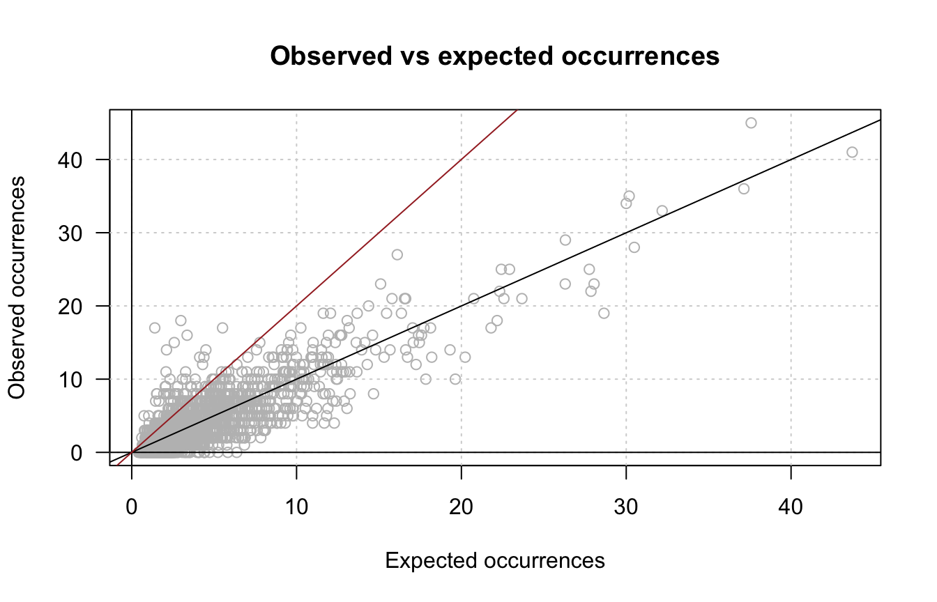
Scatter plot of observed versus expected occurrences. The black diagonal corresponds to the null hypothesis, the brown line denotes an arbitrary threshold on fold-change > 2.
- Compute the ratio between observed and expected occurrences, and draw the histogram of the ratio values, as well as a scatter plot with this ratio (Y) as a function of the expected occurrences (X).
ratio <- (x/exp.occ)

plot(exp.occ, ratio,
     col = "grey", las = 1,
     xlab = "Expected occurrences",
     ylab = "(obs/exp) ratio",
     main = "(obs/exp) ratio")
grid()
abline(h = 1, col = "black")
abline(h = 2, col = "brown")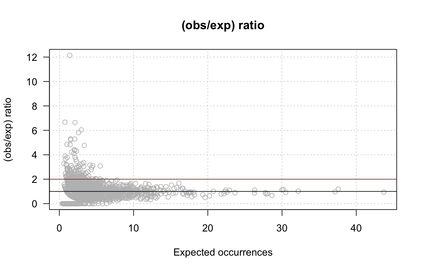
Observed/expected ratio. Top: histogram of ratio values. Bottom: ratio versus expected occurrences. The black line to the null hypothesis, the brown line denotes an arbitrary threshold on fold-change > 2.
- Compute the log-ratio of observed / expected occurrences, and draw a scatter plot with this log-ratio (Y) as a function of the expected occurrences (X).
lr <- log(x/exp.occ)
oligo.table$lr <- lr

plot(exp.occ, lr,
     col = "grey", las = 1,
     xlab = "Expected occurrences",
     ylab = "log(obs/exp)",
     main = "Log-ratio")
grid()
abline(h = 0, col = "black")
abline(h =  log(2), col = "brown")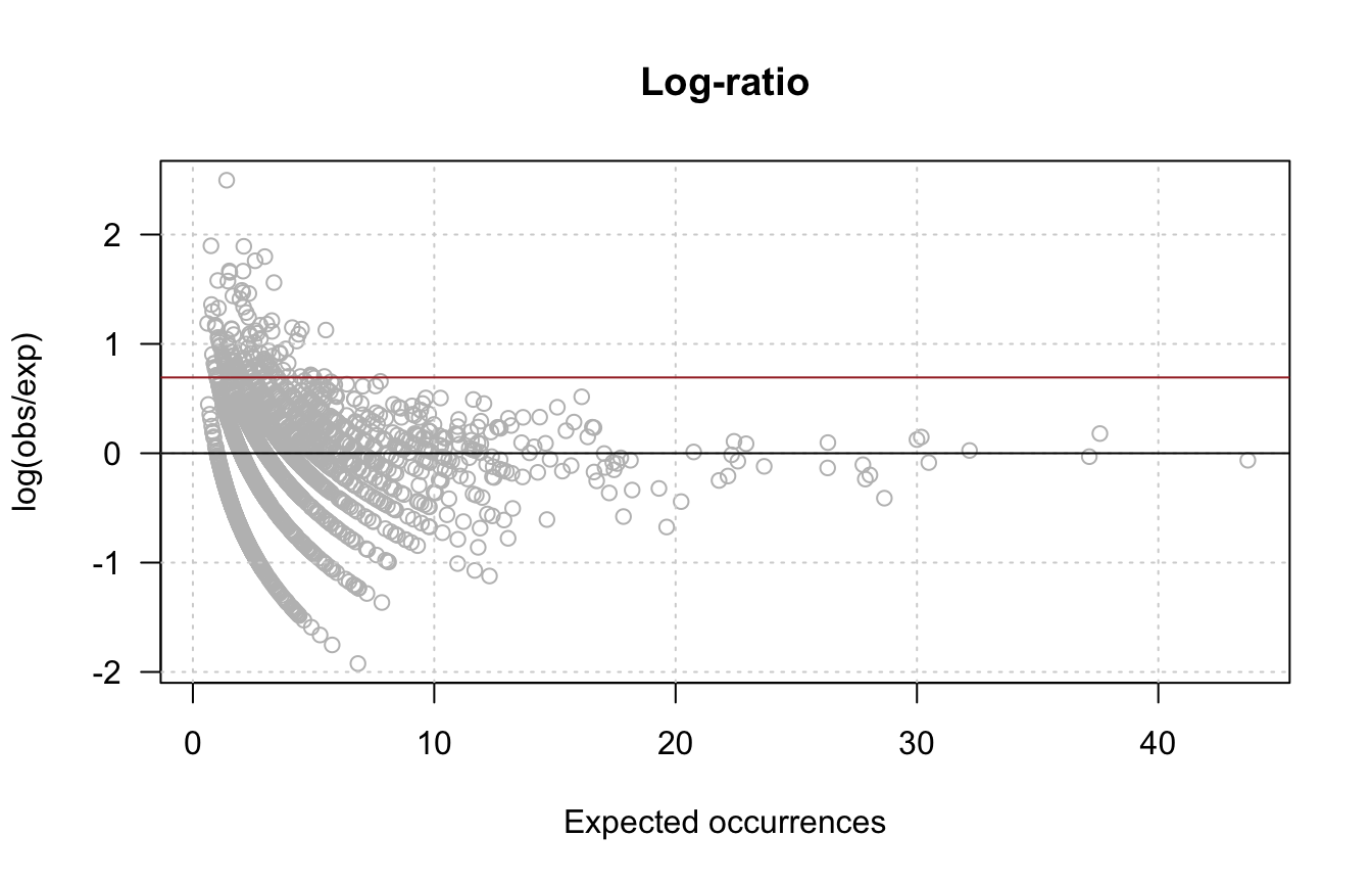
Scatter plot of observed versus expected occurrences. The black diagonal corresponds to the null hypothesis, the brown line denotes an arbitrary threshold on fold-change > 2.
\[lr = log(x/<X>)\]
- Compute the log-likelihood ratio (\(llr\)), defined below, and draw a scatter plot with this \(llr\) as a function of the expected occurrences.
\[llr = f \cdot log(x/<X>)\]
p <- oligo.table$exp_freq
llr <- p * log(x/exp.occ)
oligo.table$llr <- llr

plot(exp.occ, llr,
     col = "grey", las = 1,
     xlab = "Expected occurrences",
     ylab = "llr",
     main = "Log-likelihood ratio")
grid()
abline(h = 0, col = "black")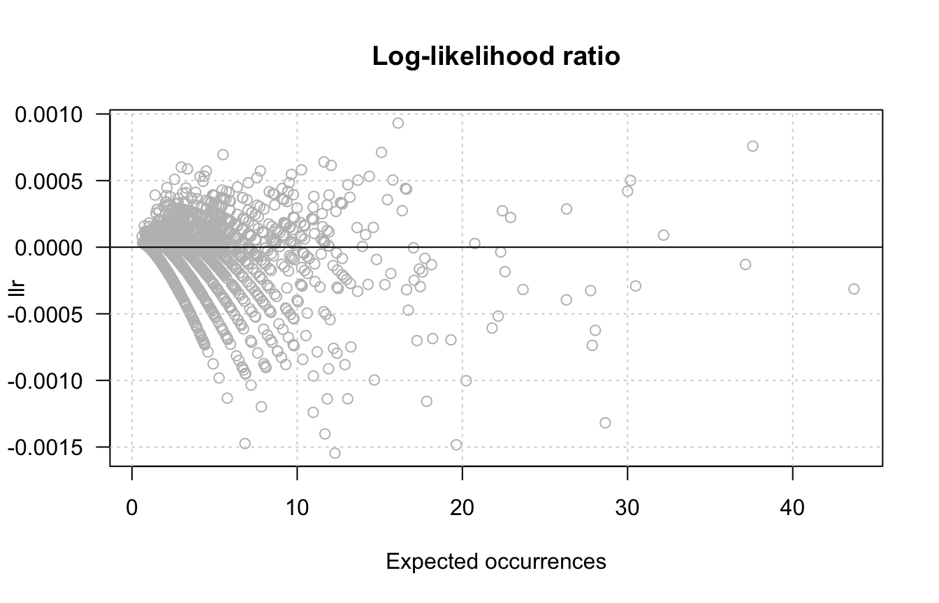
Scatter plot of log-likelihood ratio (llr) versus expected occurrences. The black line corresponds to the null hypothesis, the brown line denotes an arbitrary threshold on fold-change > 2.
# abline(h = log(2), col = "brown")Computing over-representation significance
- Draw a binomial distribution with parameters \(n = 8000\), \(p = 0.0001\).
n <- 8000
p <- 0.001
x <- 15# Number of successes
X <- 0:40 ## values to display

plot(X, dbinom(x = X, size = n, prob = p), type = "h",  col = "grey",
     ylab = "P(X = x)", las = 1,
     xlab = "X (nb of successes)")
arrows(x, 0.04, x, 0.02, lwd = 2, length = 0.1, angle = 30, col = "red")

tail <- x:40
lines(tail, dbinom(x = tail, size = n, prob = p), type = "h", col = "red")
arrows(x, 0.04, x, 0.02, lwd = 2, length = 0.1, angle = 30, col = "red")

pval <- pbinom(q = x - 1, size = n, prob = p, lower.tail = FALSE)
legend("topright", legend = paste("pval =", signif(digits = 3, pval)))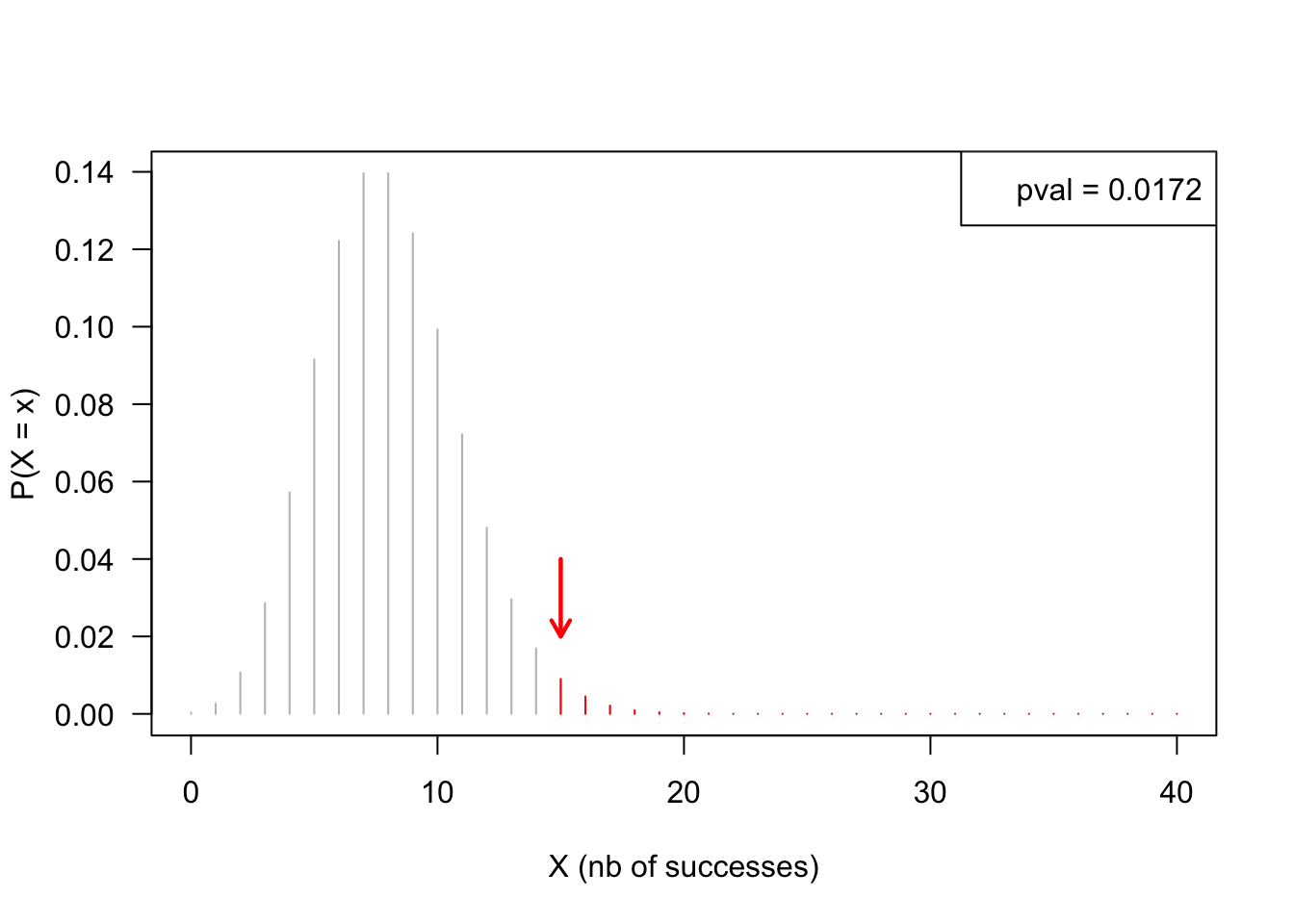
- Use the binomial distribution to compute the P-value of the observed occurrences.
\[P = T(X \ge x)\]
x <- oligo.table$occ ## Nuumber of successes
n <- sum(x)   ## Number of trials
p <- oligo.table$exp_freq ## Success probability

p <- p / sum(p) # A correction for the fact that we discarded self-overlapping occurrences
# sum(p)

nbTests <- length(x) # Number of tests

## Compute a P-value for each individual oligonucleotide
oligo.table$pval <- pbinom(q = x - 1, size = n, prob = p, lower.tail = FALSE)- Draw an histogram with the P-values of all hexanucleotides, with 20 bins.
hist(oligo.table$pval, breaks = seq(0, 1, 0.05),
     col = "beige", main = "P-value histogram")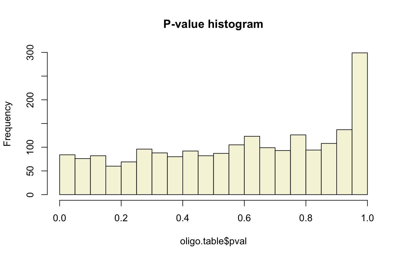
Histogram of nominal p-values for all the hexanucleotides grouped by pairs of reverse complements.
- Draw a scatter plot with the P-value (Y) as a function of the log-ratio (X).
plot(oligo.table$lr)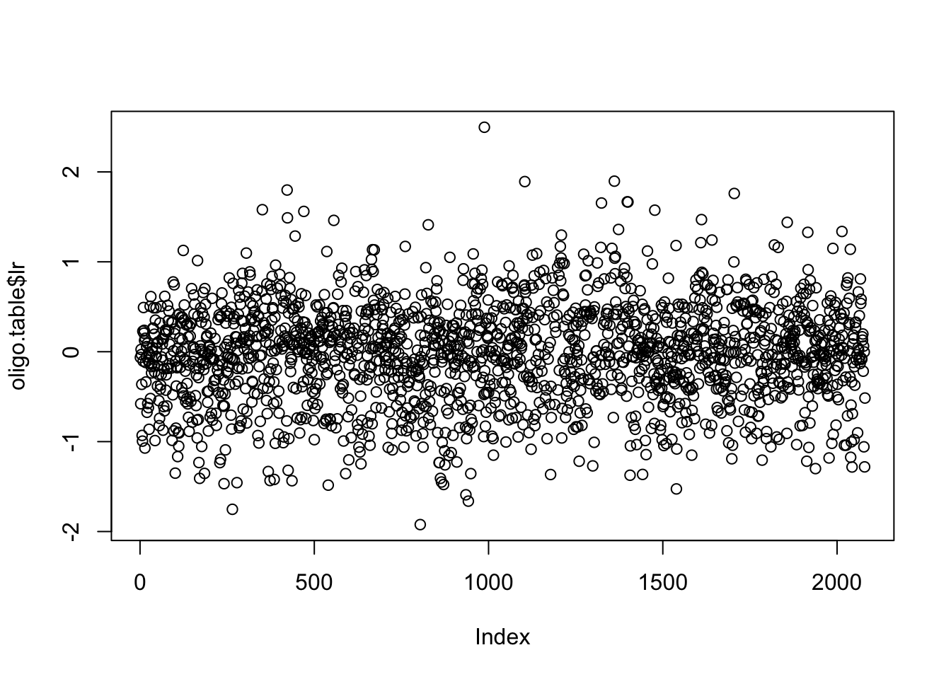
# hist(lr, breaks = 50)
plot(lr, oligo.table$pval, col = "grey", panel.first = grid())
abline(v = 0)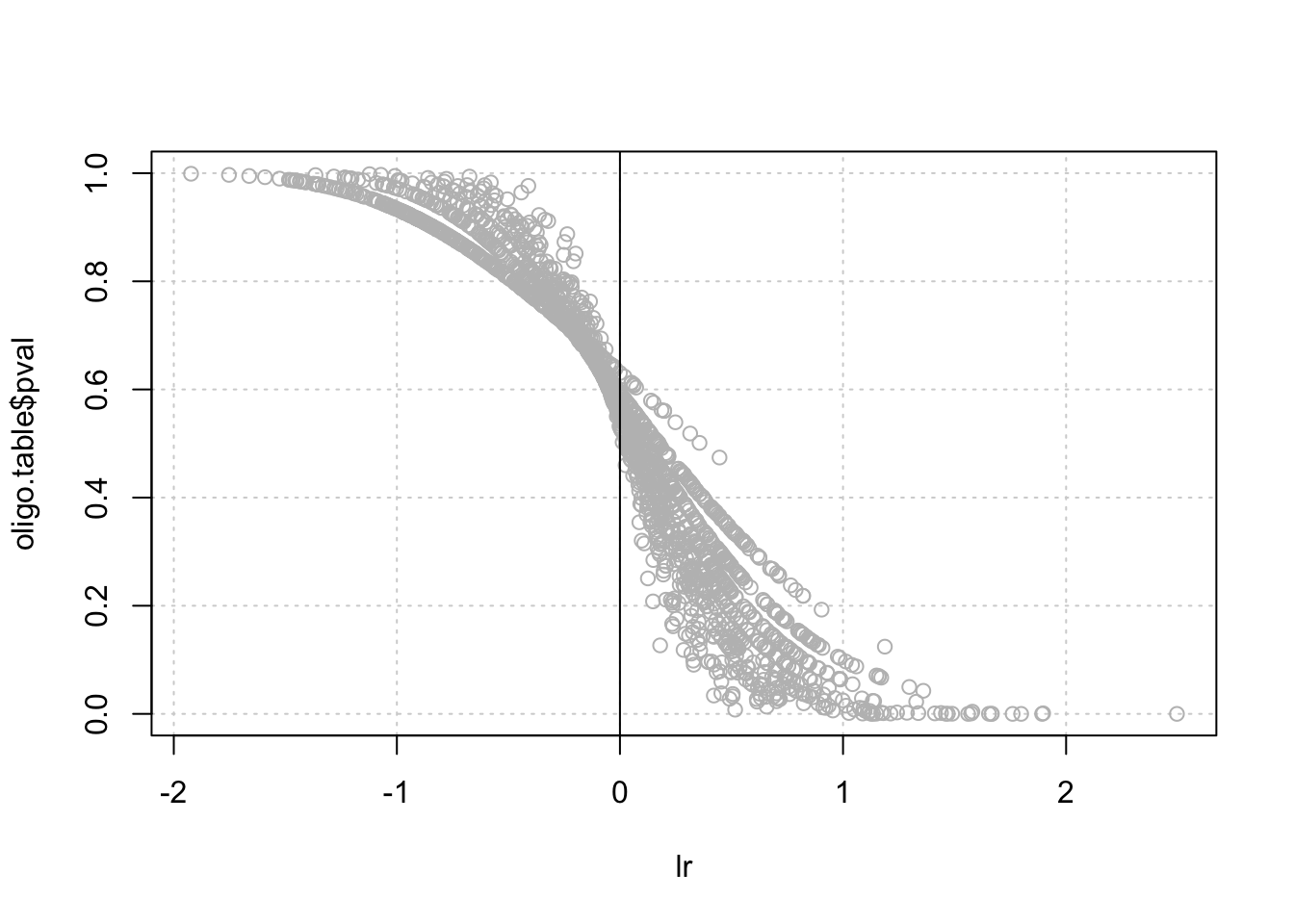
# hist(lr, breaks = 50)
plot(lr, oligo.table$pval, col = "grey",
     log = "y", las = 1, ylim = c(1e-20, 1),
     panel.first = grid())
abline(v = 0)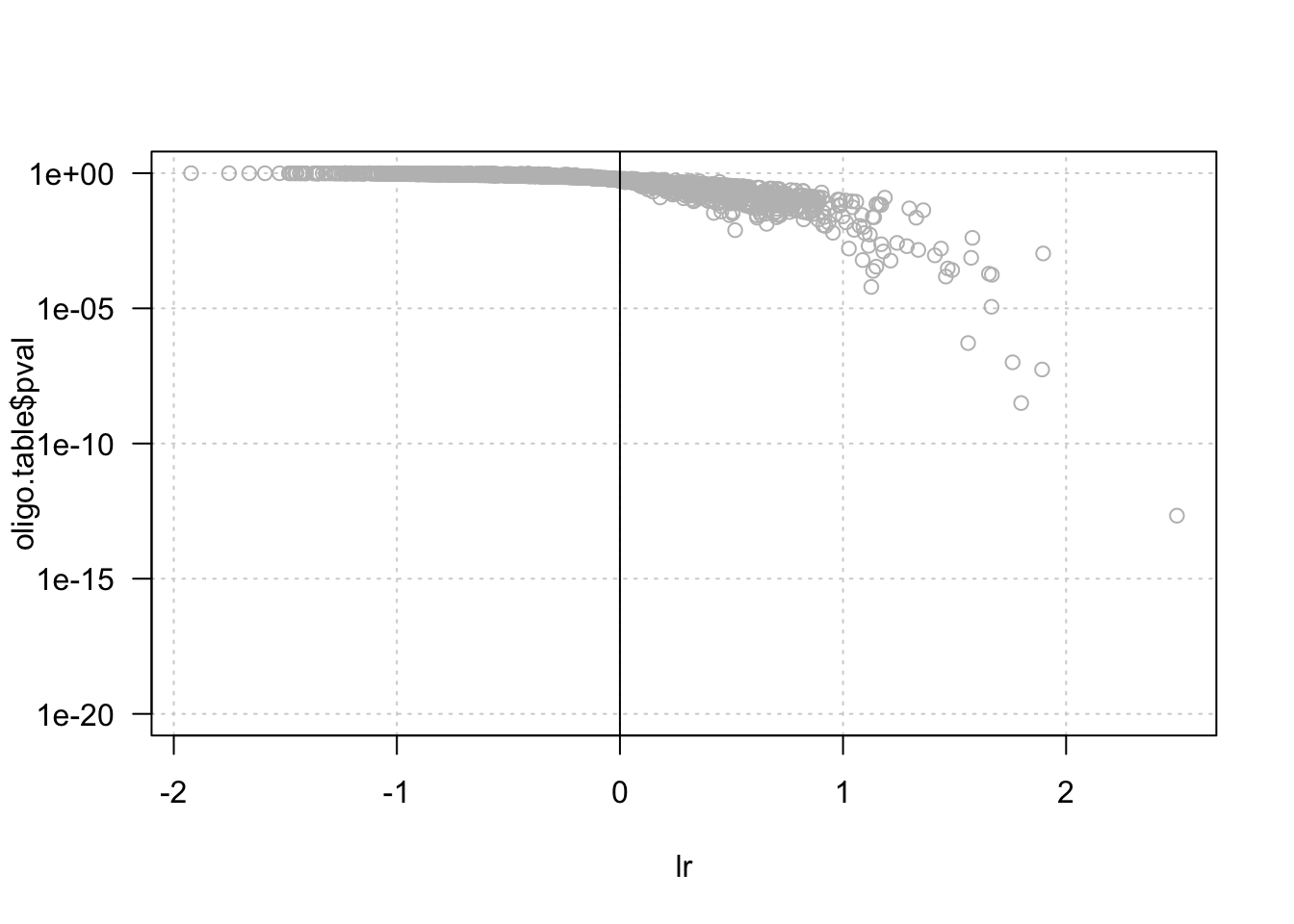
- Compute the E-value, and the significance.
\[E = P \cdot N\] \[sig = -log_{10}(E)\]
oligo.table$eval <- oligo.table$pval * nbTests
oligo.table$sig <- -log10(oligo.table$eval)- Draw a Volcano plot, with the significance as a function of the log-ratio.
plot(oligo.table$lr, oligo.table$sig,
     col = "grey",
     xlab = "Log-ratio",
     ylab = "sig = -log10(E)",
     panel.first = grid())
abline(h = 0)

alpha <- 0.05
abline(h = -log10(alpha), col = "red")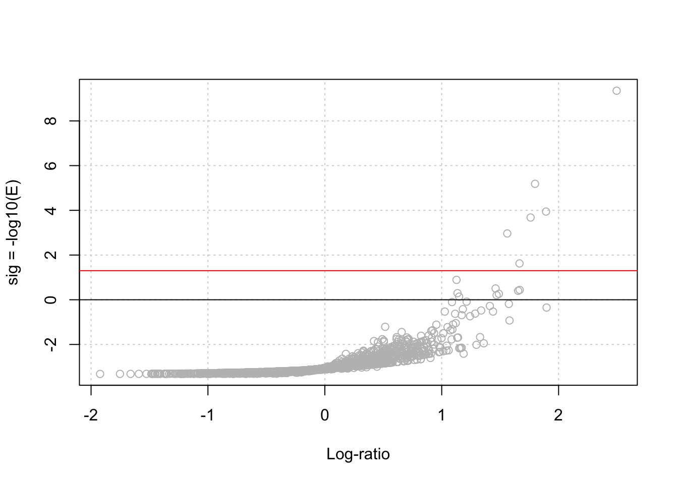
- Compute the P-value using the Poisson distribution as approximation of the binomial. Are we in suitable conditions for this approximation ? Draw a plot comparing the P-values obtained by the binomial and Poisson distributions.
lambda <- oligo.table$exp_occ * sum(oligo.table$occ) / sum(oligo.table$exp_occ)

oligo.table$pval_Poisson <- ppois(
  q = oligo.table$occ - 1, lambda = lambda, lower.tail = FALSE)

plot(oligo.table$pval, oligo.table$pval_Poisson,
     log = "xy")
abline(a  = 0, b = 1)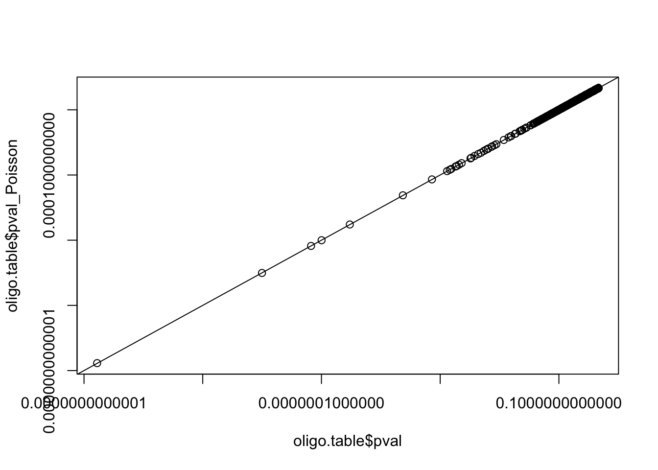
range(oligo.table$pval / oligo.table$pval_Poisson)[1] 0.9739469 1.0185630