One-to-N sequence matches in coronavirus genomes
Jacques van Helden
2021-02-16
#### General parameters for the analysis ####
reloadImage <- FALSE
quickTest <- FALSE # if True, only analyse the 2 first features


#### Sequence collection ####

## Supported:
collections <- c(
  "around-CoV-2",
  "selected",
  "around-CoV-2-plus-GISAID",
  "selected-plus-GISAID"
  )


# collection <- "around-CoV-2" # ~20 strains
# collection <- "all" # ~60 strains
# collection <- "selected" # ~50 strains
collection <- "around-CoV-2-plus-GISAID" # 16 strains
# collection <- "selected-plus-GISAID" # ~40 strains
# collection <- "all-plus-GISAID" # ~60 strains


## Choose a collection-specific path for the figures
knitr::opts_chunk$set(fig.path = paste0('figures/one-to-n-matches_', collection, '/', collection, "_"))

## Note about GIDAID sequences.
##
## A few genomes were not available in NCBI Genbank at the time of
## this analysis, and had to be downloaded from GISAID. These sequences
##  can however not be redistributed, they should thus be downloaded
##  manually to reproduce the full trees.


## Exclude incomplete genomes (i.e. those containing a lof of Ns) to avoid biases in the distance computations
excludeIncomplete <- TRUE


#### Define directories and files ####
dir <- list(main = '..')
dir$R <- file.path(dir$main, "scripts/R")

## Input directory for sequences
dir$seqdata <- file.path(dir$main, "data")
dir.create(dir$seqdata, showWarnings = FALSE, recursive = TRUE)


## Create output directory for aligned sequences
dir$results <- file.path(dir$main, "results")
dir.create(dir$results, showWarnings = FALSE, recursive = TRUE)

## Instantiate a list for output files
outfiles <- vector()

## Memory image
dir$images <- file.path(dir$main, "memory_images")
dir.create(dir$images, recursive = TRUE, showWarnings = FALSE)
outfiles["Memory image"] <- file.path(
  dir$images,
  paste0(collection, "_one-to-n_matches.Rdata"))

## Input files
infiles <- list()

## Output tables
# di$output <- file.path(dir.main, "")
# dir$tables <-

## Load custom functions
source(file.path(dir$R, "align_n_to_one.R"))
source(file.path(dir$R, "plot_pip_profiles.R"))
source(file.path(dir$R, "plot_pip_profiles_from_list.R"))

## A unequivocal pattern to identify the reference genome in the sequence names of the input file
refPattern <- "HuCoV2_WH01_2019"

## Exclude some genomes with a lot of Ns, because they bias the PIP profiles and alignments and trees
excludePatterns <- c("PnGu-P2S_2019")


#### Features of interest in the reference genome ####

features <- list()


#### Specific features  ####

## Cited from Sun et al (https://doi.org/10.1016/j.molmed.2020.02.008)in Lin et al. https://doi.org/10.20944/preprints202006.0044.v1

features[['Sun_2020']]  <- c(start = 13522, end =  23686, isCDS = FALSE)

## S1, first cleavage product of the spike protein
features[['S1']] <- c(start = 21599, end = 23617, isCDS = TRUE)

## Receptor binding domain
features[['RBD']] <- c(start = 22517, end = 23185, isCDS = TRUE)

## S2, second cleavage product of the spike protein
features[['S2']] <- c(start = 23618, end = 25381, isCDS = TRUE)


## Regions around the insertions
features[['Ins1-pm120']] <- c(start = 21647, end = 21907, isCDS = FALSE)
features[['Ins2-pm120']] <- c(start = 21899, end = 22156, isCDS = FALSE)
features[['Ins3-pm120']] <- c(start = 21899, end = 23152, isCDS = FALSE)
features[['Ins4-pm120']] <- c(start = 23483, end = 23734, isCDS = FALSE)
features[['Ins4-m240']] <- c(start = 23363, end = 23614, isCDS = FALSE)

## Receptor-binding domain

## Potential Pangolin origin after Xiao (https://doi.org/10.1101/2020.02.17.951335)
features[['Recomb-Xiao']] <- c(start = 22871, end = 23092, isCDS = FALSE)

## Recombinant region 1 seen on the PIP profiles
features[['Recomb-reg-1']] <- c(start = 2900, end = 3800, isCDS = FALSE)

## Recombinant region 2 seen on the PIP profiles
features[['Recomb-reg-2']] <- c(start = 21000, end = 24000, isCDS = FALSE)


## Recombinant region 3 seen on the PIP profiles
features[['Recomb-reg-3']] <- c(start = 27500, end = 28550, isCDS = FALSE)

## Recombinant region 4 in the RBD
## Slighty wider than Xiao's limits in order to see the context
features[['Recomb-RBD']] <- c(start = 22700, end = 23200, isCDS = FALSE)
# features[['Recomb-RBD']] <- c(start = 22760, end = 23160, isCDS = FALSE)

## Annotated coding sequences
features[['CDS-S']] <- c(start = 21563, end = 25384, isCDS = TRUE) ## Spike gene
features[['CDS-ORF3a']] <- c(start = 25393, end = 26220, isCDS = TRUE)
features[['CDS-E']] <- c(start = 26245, end = 26472, isCDS = TRUE)
features[['CDS-M']] <- c(start = 26523, end = 27191, isCDS = TRUE)
features[['CDS-ORF6']] <- c(start = 27202, end = 27387, isCDS = TRUE)
features[['CDS-ORF7a']] <- c(start = 27394, end = 27759, isCDS = TRUE)
features[['CDS-ORF8']] <- c(start = 27894, end = 28259, isCDS = TRUE)
features[['CDS-N']] <- c(start = 28274, end = 29533, isCDS = TRUE)
features[['CDS-ORF10']] <- c(start = 29558, end = 29674, isCDS = TRUE)

## Large ORF covering 2 thirds of the genome, coding for polyprotein
features[['CDS-ORF1ab']] <- c(start = 266, end = 21555, isCDS = TRUE)

## All the sequences after the big polyprotein-coding ORF1ab
features[['After-ORF1ab']] <- c(start = 21556, end = 29899, isCDS = FALSE)

## Only keep the two first features if quick test has been specified
if (quickTest) {
  features <- features[1:2]
}

## Convert feature list into a feature tbale
featureTable <- as.data.frame(t(as.data.frame.list(
  features, stringsAsFactors = FALSE)),
  row.names = names(features)  # to avoid replacement of "-" by "."
  )

# class(featureTable)
featureTable$length <- featureTable$end - featureTable$start + 1
# row.names(featureTable)
# featureTable["CDS.S", ]

featureTable <- featureTable[order(featureTable$start), ]


message("Analysing ", length(features), " features")
message("\t", paste(collapse = ", ", names(features)))

## Report the parameters
message("\tReference pattern: ", refPattern)
Strain collection: around-CoV-2-plus-GISAID
## Genome dir and files
if (length(grep(pattern = "GISAID", x = collection)) > 0) {
  useGISAID <- TRUE
  dir$sequences <- file.path(dir$main, "data", "GISAID_genomes")
  # collections <-  paste0(collections, "-plus-GISAID")
  # collection <-  paste0(collection, "-plus-GISAID")
} else {
  dir$sequences <- file.path(dir$main, "data", "genomes")
}


## Define the input sequences
infiles$sequences <- file.path(
  dir$sequences,
  paste0("genomes_", collection, ".fasta"))

## Check if the input  sequence file exists
if (!file.exists(infiles$sequences)) {
  stop("Genome sequence file is missing", "\n", infiles$sequences)
} else {
  message("Genome sequence file", "\n", infiles$sequences)
}

#### Load genome sequences ####
genomes <- readDNAStringSet(filepath = infiles$sequences, format = "fasta")

## Shorten sequence names by suppressing the fasta comment (after the space)
names(genomes) <- sub(pattern = " .*", replacement = "", x = names(genomes), perl = TRUE)

## Exclude genomes
if (excludeIncomplete) {
  excludePattern = paste0("(", paste(collapse = ")|(", excludePatterns), ")")
  excludedstrainNames <- grep(pattern = excludePattern, x = names(genomes),
                              value = TRUE, invert = FALSE)
  filteredGenomeIndices <- grep(pattern = excludePattern, x = names(genomes),
                                value = FALSE, invert = TRUE)
  message("\tExcluded ", length(excludedstrainNames)," genomes: ", paste(collapse = ", ", excludedstrainNames))
  message("\tRemaining genomes: ", length(filteredGenomeIndices))
  genomes <- genomes[filteredGenomeIndices]
# names(genomes)
}

## Report the number of genoomes
strainNames <- names(genomes)
nbStrains <- length(strainNames)
message("\tLoaded ", nbStrains, " genomes from file ", infiles$sequences)
# View(genomes)


#### Define reference and query genomes ####
refStrainName <- grep(pattern = refPattern, x = names(genomes),
                      ignore.case = TRUE, value = TRUE)
if (is.null(refStrainName)) {
  stop("Could not identify reference genome with pattern ", refPattern)
}
message("\tReference genome name: ", refStrainName)Parameters
#### Define a list of parameters ####
parameters <- list()
parameters$collection <- collection
parameters$refStrainName <- refStrainName
parameters$nbStrains <- nbStrains
parameters$sequenceDir <- dir$sequences
parameters$sequenceFile <- infiles$sequences
parameters$memoryImage <- outfiles["Memory image"]


## Exclude metagenomic assemblies
parameters$pasDeTambouille <- FALSE
if (parameters$pasDeTambouille) {
  excludePatterns <- append(excludePatterns, "BtYu-RmYN02_2019")
}

kable(t(as.data.frame.list(parameters)),
      caption = "Parameters of the analysis",
col.names = "Parameter")| Parameter | |
|---|---|
| collection | around-CoV-2-plus-GISAID |
| refStrainName | HuCoV2_WH01_2019 |
| nbStrains | 25 |
| sequenceDir | ../data/GISAID_genomes |
| sequenceFile | ../data/GISAID_genomes/genomes_around-CoV-2-plus-GISAID.fasta |
| memoryImage | ../memory_images/around-CoV-2-plus-GISAID_one-to-n_matches.Rdata |
| pasDeTambouille | FALSE |
Strain statistics
#### Compute statistics about sequence sizes ###
strainStats <- data.frame(
  n = 1:length(genomes),
  row.names = names(genomes),
  status = rep("Query", length.out = length(strainNames))
)
strainStats[,"status"] <- as.vector(strainStats[,"status"])
strainStats[refStrainName,"status"] <- "Reference"
g <- 1
for (g in strainNames) {
  strainStats[g, "length"] <- length(genomes[[g]])
}
#### Define the color associated to each sequence ####
## Color palette per species
speciesPalette <- list(
Human = "#880000",
Bat = "#888888",
Pangolin = "#447700",
Camel = "#BB8800",
Pig = "#FFBBBB",
Civet = "#00BBFF"
)
## Species prefix in the tip labels
speciesPrefix <- c("Hu" = "Human",
"Bt" = "Bat",
"Pn" = "Pangolin",
"Cm" = "Camel",
"Pi" = "Pig",
"Cv" = "Civet")
## Strain-specific colors
strainColor <- c(
"HuCoV2_WH01_2019" = "red",
"HuSARS-Frankfurt-1_2003" = "#0044BB",
"PnGu1_2019" = "#00CC00",
"PnMP789" = "#00FF88",
"BtRaTG13_" = "#FF6600",
"BtYu-RmYN" = "#FFBB22",
"BtZXC21" = "black",
"BtZC45" = "black")
## Identify species per tip
for (prefix in names(speciesPrefix)) {
strainStats[grep(pattern = paste0("^", prefix), x = row.names(strainStats), perl = TRUE), "species"] <- speciesPrefix[prefix]
}
## Assign acolor to each species
strainStats$color <- "grey" # default
strainStats$color <- speciesPalette[as.vector(strainStats$species)]
for (strain in names(strainColor)) {
strainStats[grep(pattern = paste0("^", strain),
x = row.names(strainStats), perl = TRUE), "color"] <- strainColor[strain]
}
## Assign specific color to some nodes
## Define a color for each strain
strainColors <- (unlist(strainStats$color))
names(strainColors) <- row.names(strainStats)| n | status | length | species | color | |
|---|---|---|---|---|---|
| BtBM48-31 | 1 | Query | 29276 | Bat | #888888 |
| BtGX2013 | 2 | Query | 29161 | Bat | #888888 |
| BtHKU3-12 | 3 | Query | 29704 | Bat | #888888 |
| BtRaTG13_2013_Yunnan | 4 | Query | 29855 | Bat | #FF6600 |
| BtRs4874 | 5 | Query | 30311 | Bat | #888888 |
| BtYN2013 | 6 | Query | 29142 | Bat | #888888 |
| BtYN2018B | 7 | Query | 30256 | Bat | #888888 |
| BtZC45 | 8 | Query | 29802 | Bat | black |
| BtZXC21 | 9 | Query | 29732 | Bat | black |
| Cv007-2004 | 10 | Query | 29540 | Civet | #00BBFF |
| HuCoV2_WH01_2019 | 11 | Reference | 29899 | Human | red |
| HuSARS-Frankfurt-1_2003 | 12 | Query | 29727 | Human | #0044BB |
| PnGX-P1E_2017 | 13 | Query | 29801 | Pangolin | #447700 |
| PnGX-P2V_2018 | 14 | Query | 29795 | Pangolin | #447700 |
| PnMP789 | 15 | Query | 29521 | Pangolin | #00FF88 |
| BtRc-o319 | 16 | Query | 29718 | Bat | #888888 |
| BtRacCS203 | 17 | Query | 29832 | Bat | #888888 |
| BtRacCS264 | 18 | Query | 29820 | Bat | #888888 |
| BtRacCS253 | 19 | Query | 29820 | Bat | #888888 |
| BtRacCS224 | 20 | Query | 29820 | Bat | #888888 |
| BtRacCS271 | 21 | Query | 29820 | Bat | #888888 |
| BtYu-RmYN02_2019 | 22 | Query | 29671 | Bat | #FFBB22 |
| PnGu1_2019 | 23 | Query | 29825 | Pangolin | #00CC00 |
| BtCambodia/RShSTT200/2010 | 24 | Query | 29793 | Bat | #888888 |
| BtCambodia/RShSTT182/2010 | 25 | Query | 29787 | Bat | #888888 |
The collection around-CoV-2-plus-GISAID contains 25 virus genome sequences.
Features
| start | end | isCDS | length | |
|---|---|---|---|---|
| CDS-ORF1ab | 266 | 21555 | 1 | 21290 |
| Recomb-reg-1 | 2900 | 3800 | 0 | 901 |
| Sun_2020 | 13522 | 23686 | 0 | 10165 |
| Recomb-reg-2 | 21000 | 24000 | 0 | 3001 |
| After-ORF1ab | 21556 | 29899 | 0 | 8344 |
| CDS-S | 21563 | 25384 | 1 | 3822 |
| S1 | 21599 | 23617 | 1 | 2019 |
| Ins1-pm120 | 21647 | 21907 | 0 | 261 |
| Ins2-pm120 | 21899 | 22156 | 0 | 258 |
| Ins3-pm120 | 21899 | 23152 | 0 | 1254 |
| RBD | 22517 | 23185 | 1 | 669 |
| Recomb-RBD | 22700 | 23200 | 0 | 501 |
| Recomb-Xiao | 22871 | 23092 | 0 | 222 |
| Ins4-m240 | 23363 | 23614 | 0 | 252 |
| Ins4-pm120 | 23483 | 23734 | 0 | 252 |
| S2 | 23618 | 25381 | 1 | 1764 |
| CDS-ORF3a | 25393 | 26220 | 1 | 828 |
| CDS-E | 26245 | 26472 | 1 | 228 |
| CDS-M | 26523 | 27191 | 1 | 669 |
| CDS-ORF6 | 27202 | 27387 | 1 | 186 |
| CDS-ORF7a | 27394 | 27759 | 1 | 366 |
| Recomb-reg-3 | 27500 | 28550 | 0 | 1051 |
| CDS-ORF8 | 27894 | 28259 | 1 | 366 |
| CDS-N | 28274 | 29533 | 1 | 1260 |
| CDS-ORF10 | 29558 | 29674 | 1 | 117 |
Feature matches and alignments
We perform a global pairwise alignment (Needle-Waterman algorithm) between each feature of the reference strain (HuCoV2_WH01_2019) and each one of the query genomes.
The collected nucleic sequences are then aligned based on their translated sequences. This ensures a more relevant placing of the gaps. These translation-based alignments are exported in aminoacids and DNA formats (the DNA sequences are obtained by reverse-mapping the aligned aminoacid sequences onto the input DNA sequences).
For each alignment (AA and DNA) wee compute a consensus matrix, indicating the frequency of each residue (row of the consensus matrix) in each position of the alignment (column of the matrix).
#### One-to-N alignmemnt of user-speficied genomic features ####


i <- 1
testFeature <- "Recomb-RBD"
i <- which(names(features) == testFeature)

## Rune one-ton matches and translation-based mumti^ple alignment + PIP profiles
for (i in 1:length(features)) {
  featureName <- names(features)[i]

  ## Compute feature length
  featureLimits <- features[[featureName]]
  featureStart <- featureLimits[["start"]]
  featureEnd <- featureLimits[["end"]]
  featureLength <-
    featureEnd - featureStart  + 1

  message("Searching matches for feature ",
          i, "/", length(features), "\t",
          featureName,
          " (", featureLimits[1], "-", featureLimits[2], ")",
          " in collection ", collection)

  ## Print a section title with the feature name and limits
  cat(sep = "", "\n### ",  featureName,
      " (", featureLimits[1], "-", featureLimits[2],
      "; ", featureLength,"bp)", "\n")


  ## Choose a collection- and feature-specific path for the figures
  knitr::opts_chunk$set(fig.path = paste0(
    'figures/one-to-n-matches_', collection, '/',
    collection, '_vs_', featureName))


  #### Define feature-specific output directory ####
  featurePrefix <- paste0(
    featureName,
    "_", collection)

  dir[[featureName]] <- file.path(dir$results, featurePrefix)
  message("\tOutput directory: ", dir[[featureName]] )
  dir.create(dir[[featureName]], showWarnings = FALSE, recursive = TRUE)

  #### Find feature matches by 1-to-1 alignment with each genome ####

  ## Define output file for unaligned matching sequences
  outfiles[paste0(featurePrefix, "_matches")]  <- file.path(
    dir[[featureName]], paste0(featurePrefix, "_matches.fasta"))
  message("\tMatching sequences: ",
          outfiles[paste0(featurePrefix, "_matches")])

  ## Get sequence of the feature from the reference genome
  refSeq <- subseq(genomes[refStrainName],
                   start = featureLimits[1],
                   end = featureLimits[2])

  ## Match the reference feature with all the genomes
  if (reloadImage) {
    featureAlignmentsNto1 <- allFeatureAlignments[[featureName]]
  } else {
    featureAlignmentsNto1 <- alignNtoOne(
      refSequence = refSeq,
      querySequences = genomes,
      type = "global-local",
      outfile = outfiles[paste0(featurePrefix, "_matches")])
    allFeatureAlignments[[featureName]] <- featureAlignmentsNto1

  }


  #### Translation-based alignments ####
  if (featureTable[featureName, "isCDS"]) {
    message("\tTranslation-based multiple alignment of feature ", featureName, "; DNA output")

    #### Align translated sequenecs and return correponding nucleic sequences ####
    featureAlignmentsNto1$tralignedDNA <- AlignTranslation(
      DNAStringSet(featureAlignmentsNto1$sequences),
      type = "DNAStringSet",
      verbose = FALSE)

    ## Save multiple-aligned DNA sequences
    outfiles[paste0(featurePrefix, "_tralignedDNA")]  <- file.path(
      dir[[featureName]], paste0(featurePrefix, "_tralignedDNA.fasta"))
    message("\tTranslation-based alignment saved in file ",
            outfiles[paste0(featurePrefix, "_tralignedDNA")])
    writeXStringSet(
      x = featureAlignmentsNto1$tralignedDNA,
      filepath = outfiles[paste0(featurePrefix, "_tralignedDNA")] )

    ## Convert alignment to position-weight matrix
    featureAlignmentsNto1$tralignedDNAConsensus <- consensusMatrix(
      x = featureAlignmentsNto1$tralignedDNA)

    #### Align translated sequenecs and return correponding AA sequences ####
    message("\tTranslation-based multiple alignment of feature ", featureName, "; AA output")
    featureAlignmentsNto1$tralignedAA <- AlignTranslation(
      DNAStringSet(featureAlignmentsNto1$sequences),
      type = "AAStringSet",
      verbose = FALSE)

    ## Convert alignment to position-weight matrix
    featureAlignmentsNto1$tralignedAAConsensus <- consensusMatrix(
      x = featureAlignmentsNto1$tralignedAA)

    ## Save multiple-aligned AA sequences
    outfiles[paste0(featurePrefix, "_tralignedAA")]  <- file.path(
      dir[[featureName]], paste0(featurePrefix, "_tralignedAA.fasta"))
    message("\tTranslation-based alignment saved in file ",
            outfiles[paste0(featurePrefix, "_tralignedAA")])
    writeXStringSet(
      x = featureAlignmentsNto1$tralignedAA,
      filepath = outfiles[paste0(featurePrefix, "_tralignedAA")] )
  }

  ## Compute sequence order by decreasing PIP score
  seqOrder <- order(featureAlignmentsNto1$stat$score, decreasing = TRUE)


  ## Print matching statistics
  kable(featureAlignmentsNto1$stats[seqOrder, ],
        caption = paste0(
          "One-to-N alignment of feature ",
          featureName))

  #### PIP profiles ####
  ## Choose window size
  if (featureLength > 20000) {
    windowSize <- 800
  } else if (featureLength > 5000) {
    windowSize <- 500
  } else if (featureLength > 3000) {
    windowSize <- 200
  } else if (featureLength > 400) {
    windowSize <- 100
  } else {
    windowSize <- max(50, 10 * round(featureLength / 100))
  }


  ## DNA PIP profile of one-to-N alignment
  PlotPIPprofilesFromList(
#    alignments = featureAlignmentsNto1$alignments[seqOrder],
    alignments = featureAlignmentsNto1$alignments,
    reversePlot = TRUE,
    windowSize = windowSize,
    main = paste0("PIP profiles: collection ", collection,
                  "\nGenomic feature ", featureName, " (", featureStart, ":", featureEnd ,", ", featureLength, " bp)"),
    #    colors = NULL,
    colors = strainColors,
    legendMargin = 0.25,
    legendCorner = "topright",
    lwd = 1,
    legendCex = 0.5,
    ylim = c(30, 100))

  ## Identify the correspodences between matches and sequences
  seqNames <- names(featureAlignmentsNto1$alignments)
  refSeqName <- refStrainName
  matchNames <- names(featureAlignmentsNto1$sequences)
  refMatchName <- grep(pattern = paste0("^", refStrainName), matchNames,
                       perl = TRUE, value = TRUE)

  ## Define colors
  matchColors <- strainColors[seqNames]
  names(matchColors) <- matchNames

  if (featureTable[featureName, "isCDS"]) {

    #### DNA PIP profile of translation-based multiple alignment ####
    PlotPIPprofiles(
      alignment = featureAlignmentsNto1$tralignedDNA,
      refSeqName = refMatchName,
      plotRefGaps = FALSE,
      reversePlot = TRUE,
      windowSize = windowSize,
      main = paste0("DNA PIP profiles – collection: ", collection,
                    "\nGenomic feature ", featureName, " (", featureStart, ":", featureEnd ,", ", featureLength, " bp)"),
      colors = matchColors,
      legendMargin = 0.3,
      legendCorner = "topright",
      lwd = 1,
      legendCex = 0.5,
      ylim = c(30, 100))

    ## AA PIP profile of translation-based multiple alignment
    PlotPIPprofiles(
      #    alignments = featureAlignmentsNto1$alignments[seqOrder],
      alignment = featureAlignmentsNto1$tralignedAA,
      refSeqName = refMatchName,
      plotRefGaps = FALSE,
      reversePlot = TRUE,
      windowSize = windowSize/3,
      main = paste0("AA PIP profiles: collection ", collection,
                    "\nGenomic feature ", featureName, " (", featureStart, ":", featureEnd ,", ", featureLength, " bp)"),
      colors = matchColors,
      legendMargin = 0.3,
      legendCorner = "topright",
      lwd = 1,
      legendCex = 0.5,
      ylim = c(30, 100))
  }


}
Sun_2020 (13522-23686; 10165bp)
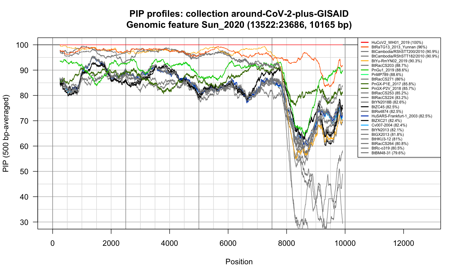
Feature-specific Percent Identical Positions (PIP) profiles.
S1 (21599-23617; 2019bp)
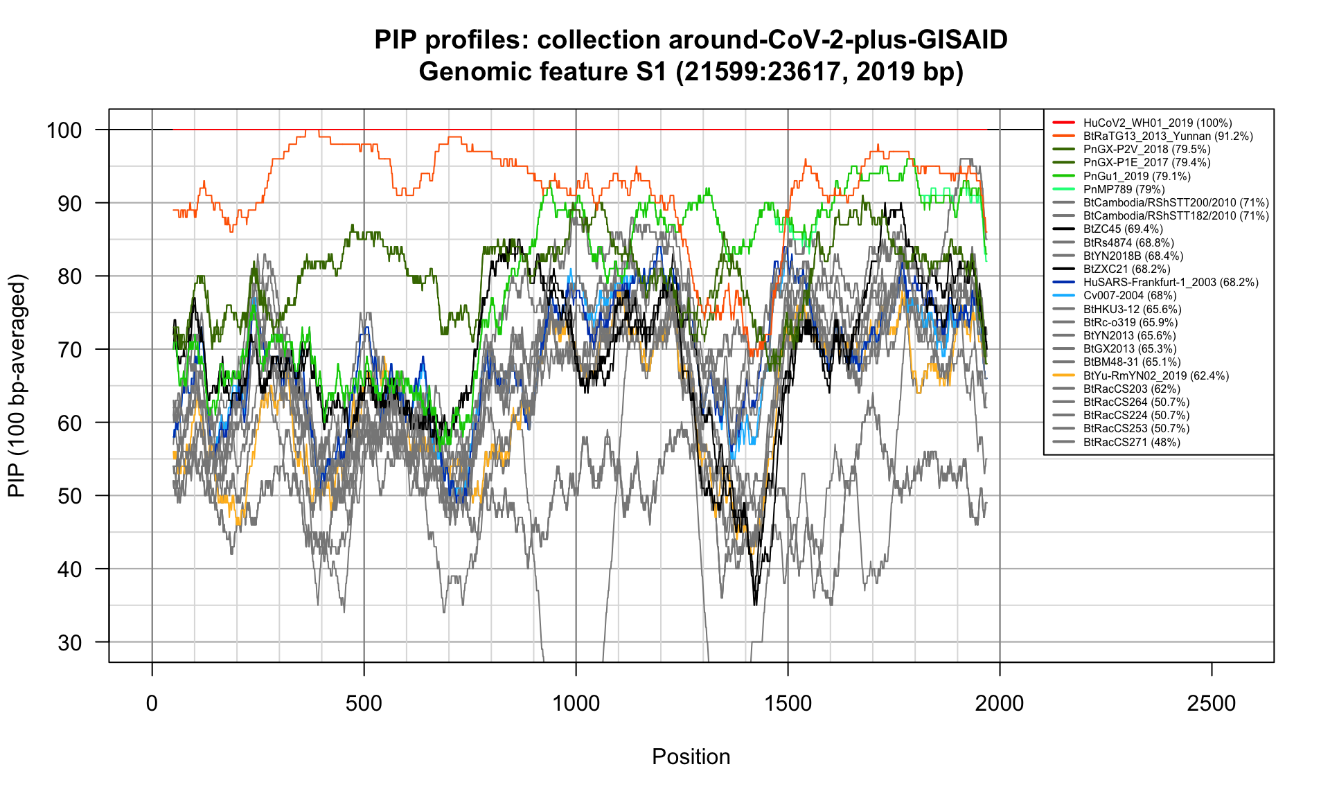
Feature-specific Percent Identical Positions (PIP) profiles.
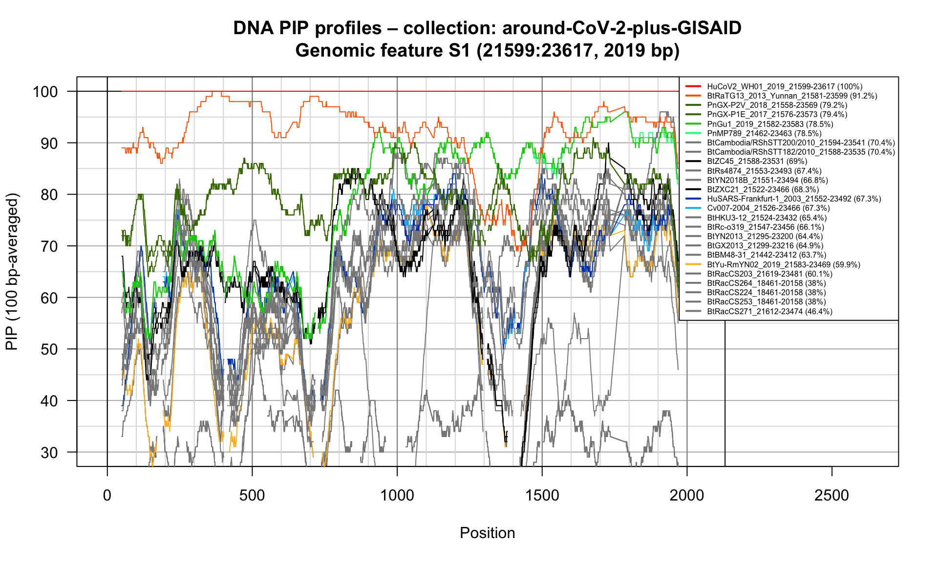
Feature-specific Percent Identical Positions (PIP) profiles.
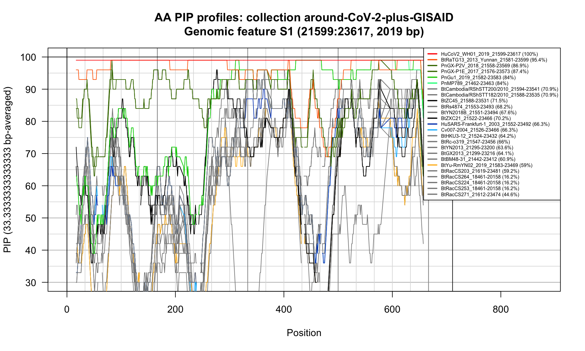
Feature-specific Percent Identical Positions (PIP) profiles.
RBD (22517-23185; 669bp)
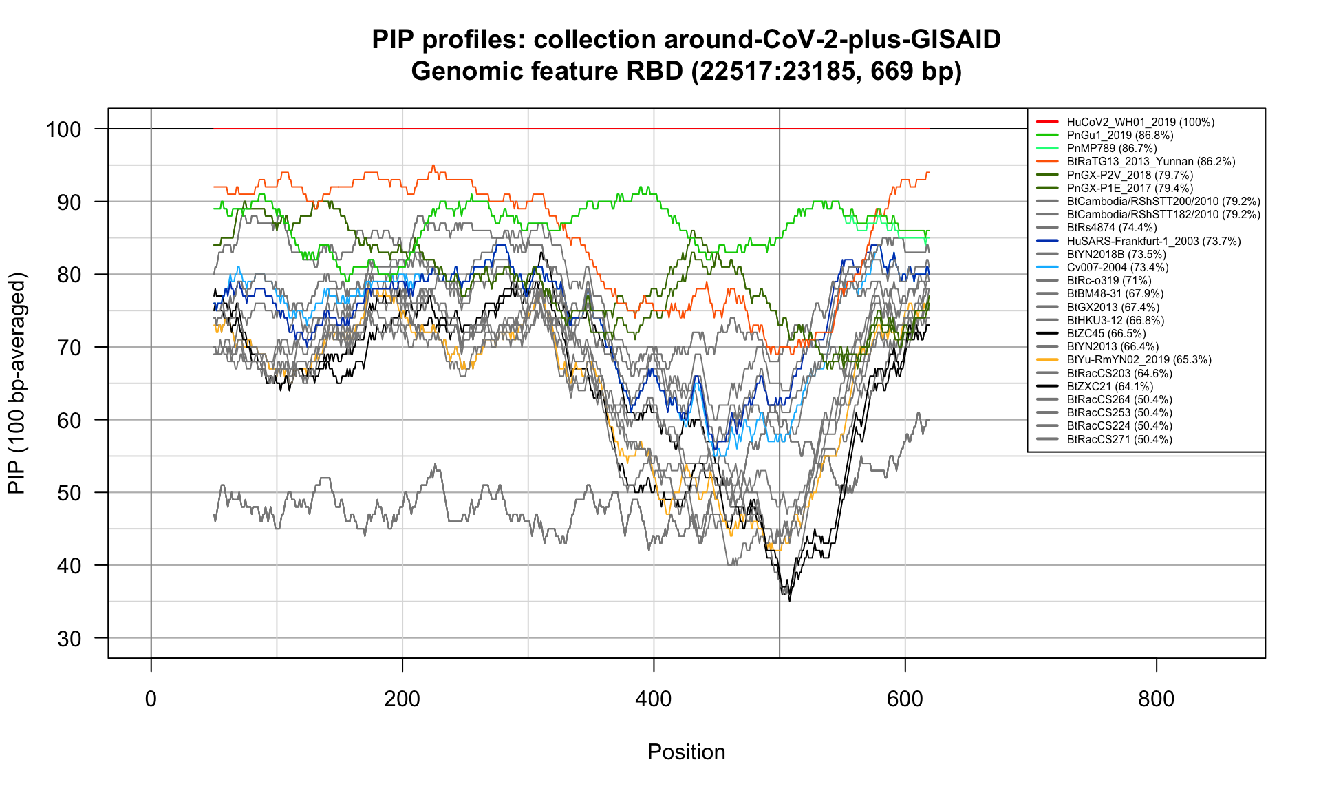
Feature-specific Percent Identical Positions (PIP) profiles.
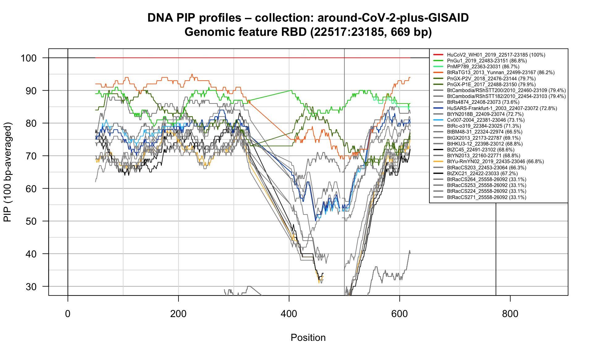
Feature-specific Percent Identical Positions (PIP) profiles.
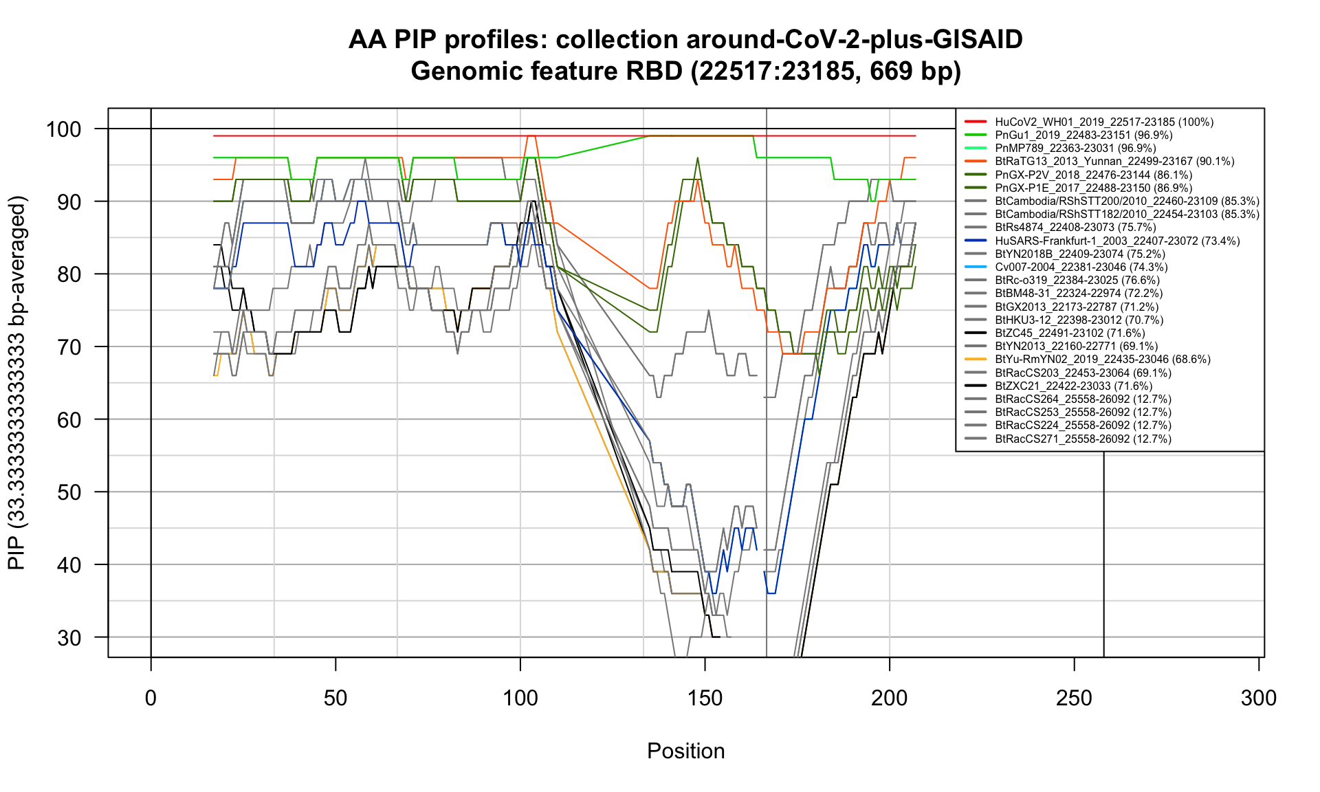
Feature-specific Percent Identical Positions (PIP) profiles.
S2 (23618-25381; 1764bp)
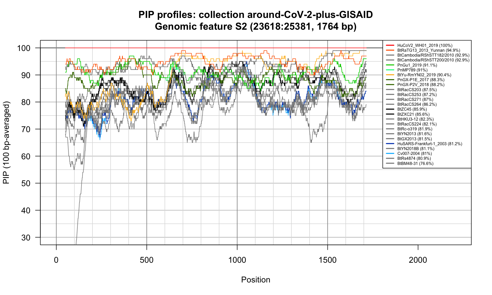
Feature-specific Percent Identical Positions (PIP) profiles.
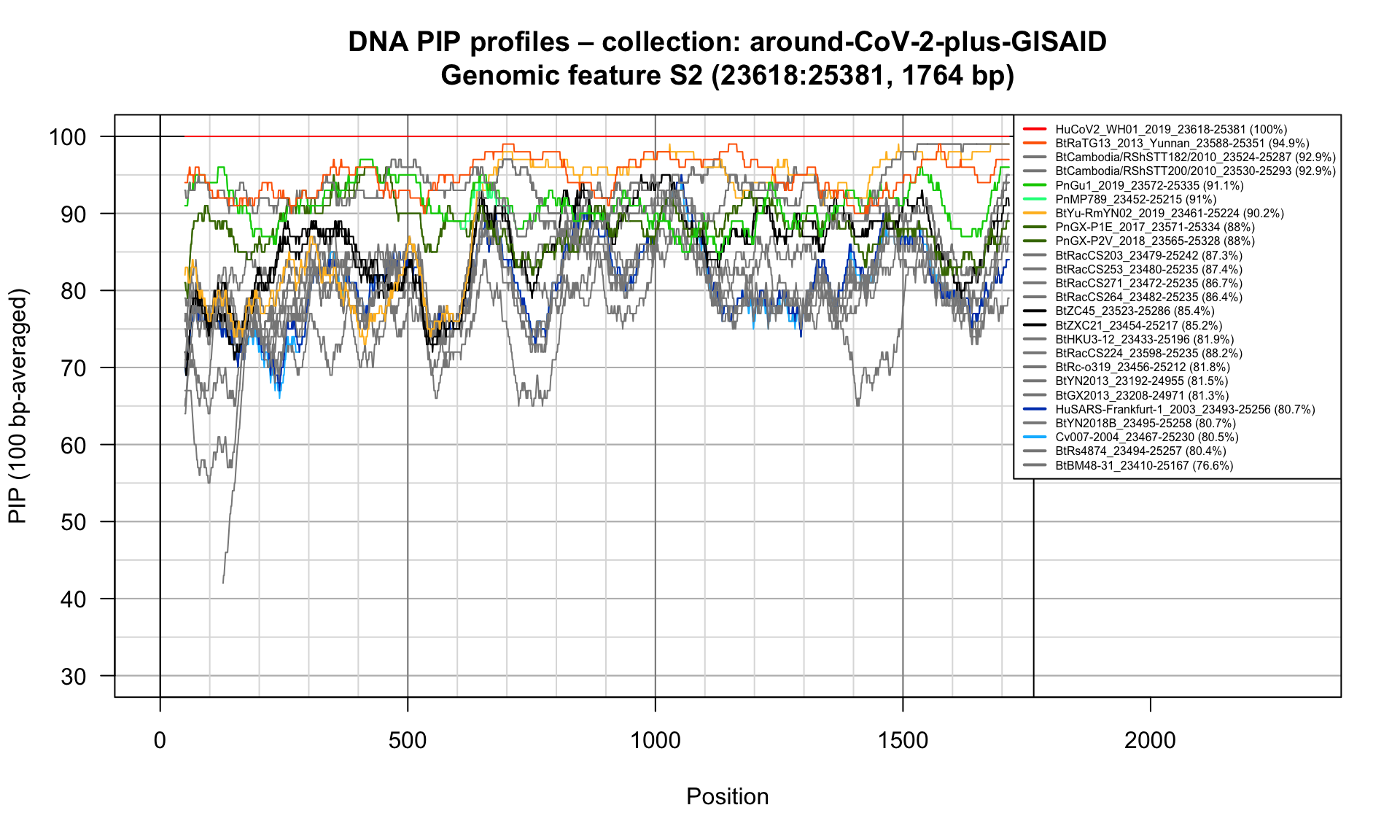
Feature-specific Percent Identical Positions (PIP) profiles.
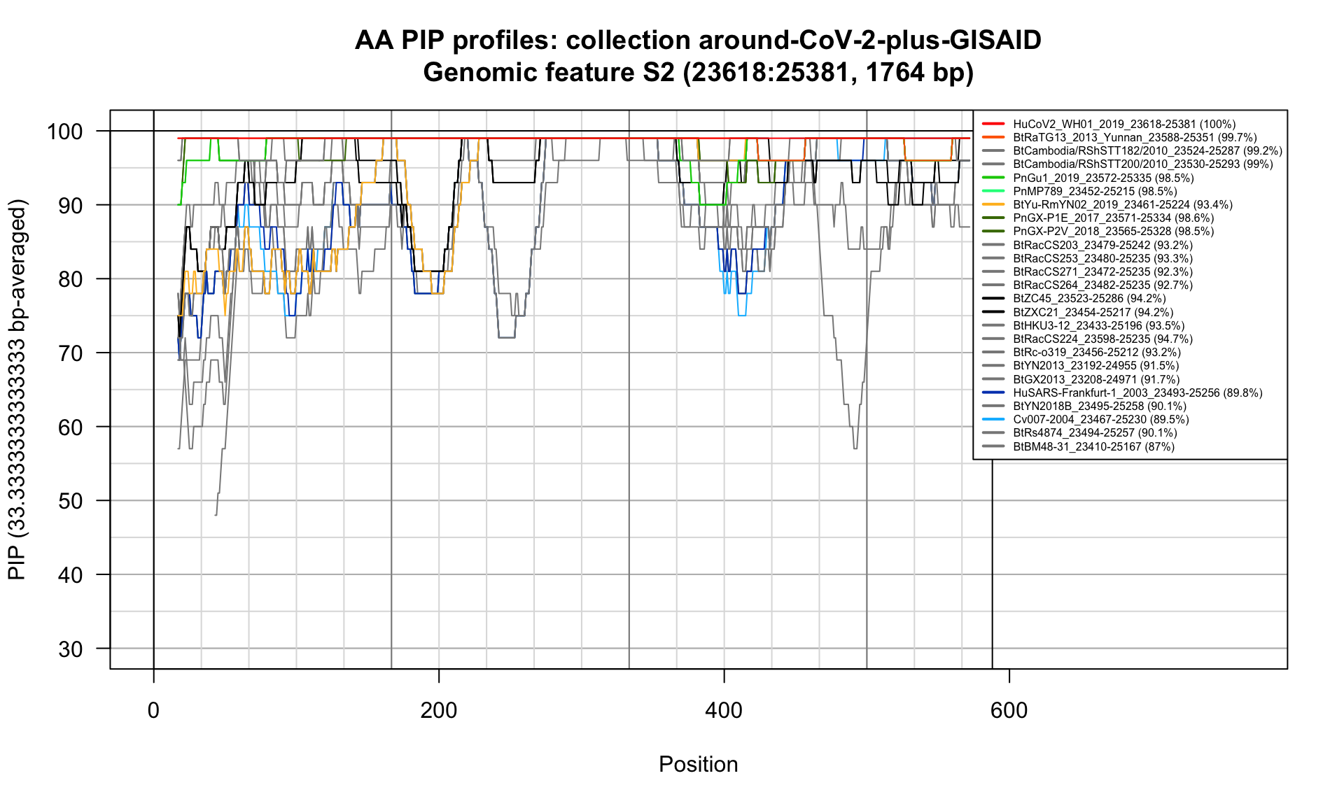
Feature-specific Percent Identical Positions (PIP) profiles.
Ins1-pm120 (21647-21907; 261bp)
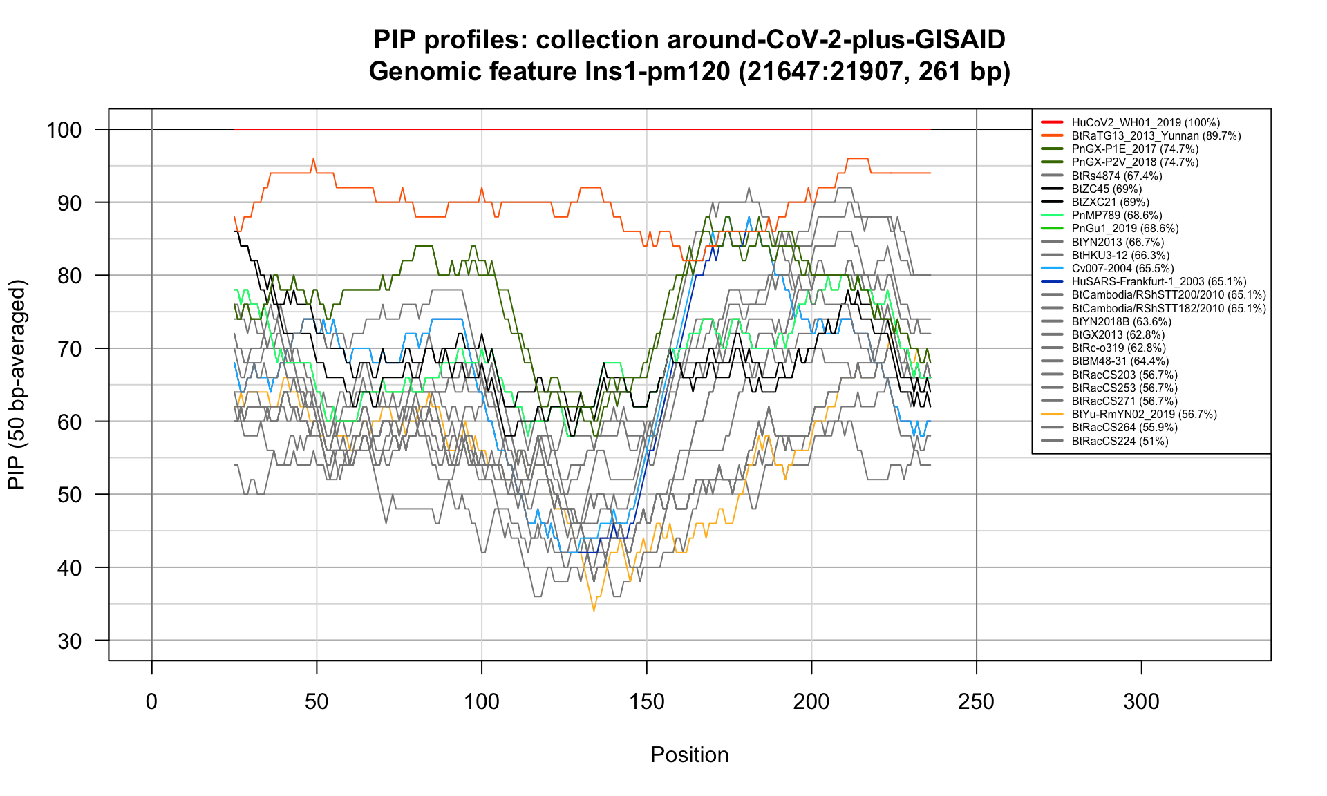
Feature-specific Percent Identical Positions (PIP) profiles.
Ins2-pm120 (21899-22156; 258bp)
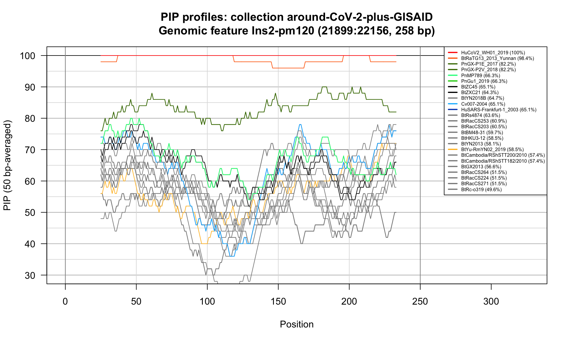
Feature-specific Percent Identical Positions (PIP) profiles.
Ins3-pm120 (21899-23152; 1254bp)
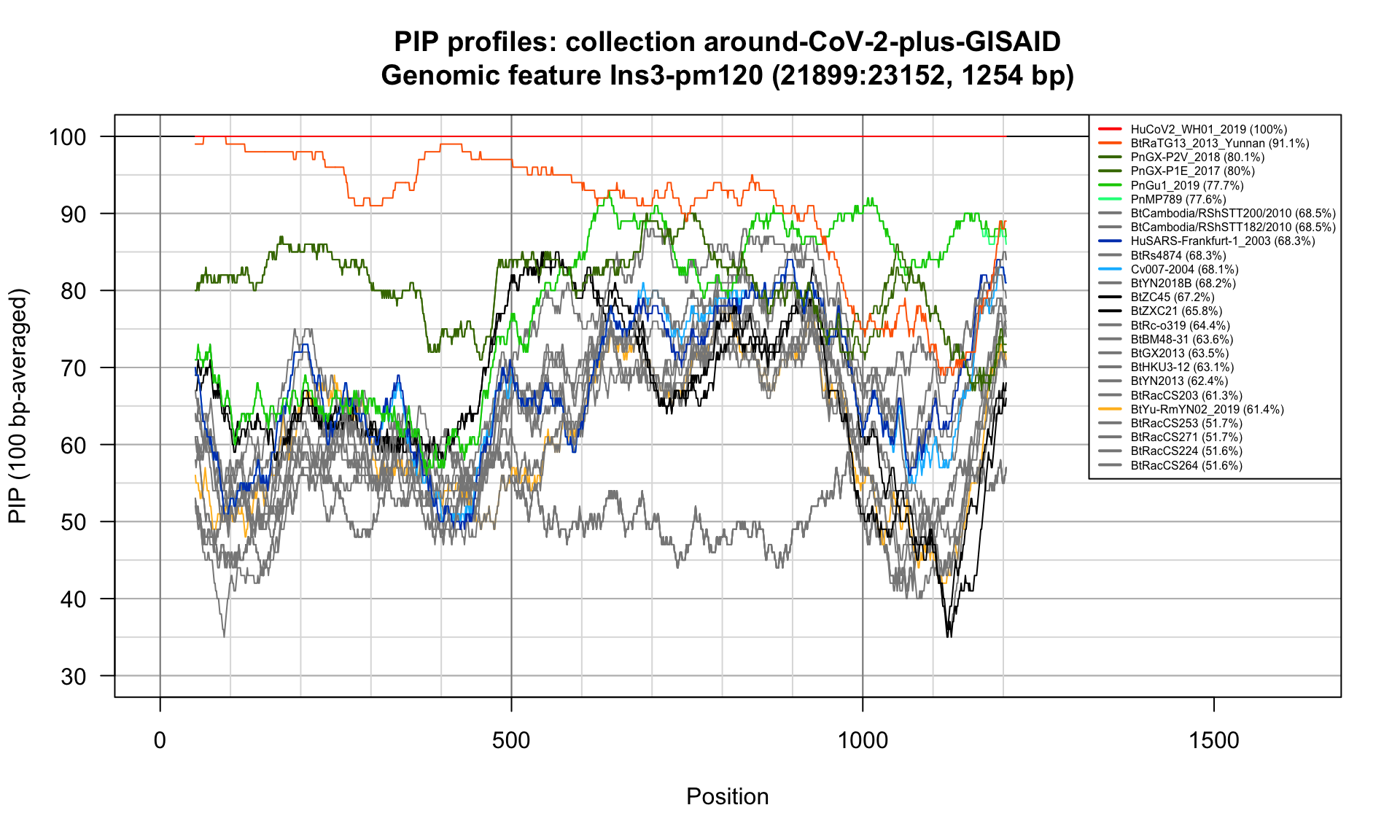
Feature-specific Percent Identical Positions (PIP) profiles.
Ins4-pm120 (23483-23734; 252bp)
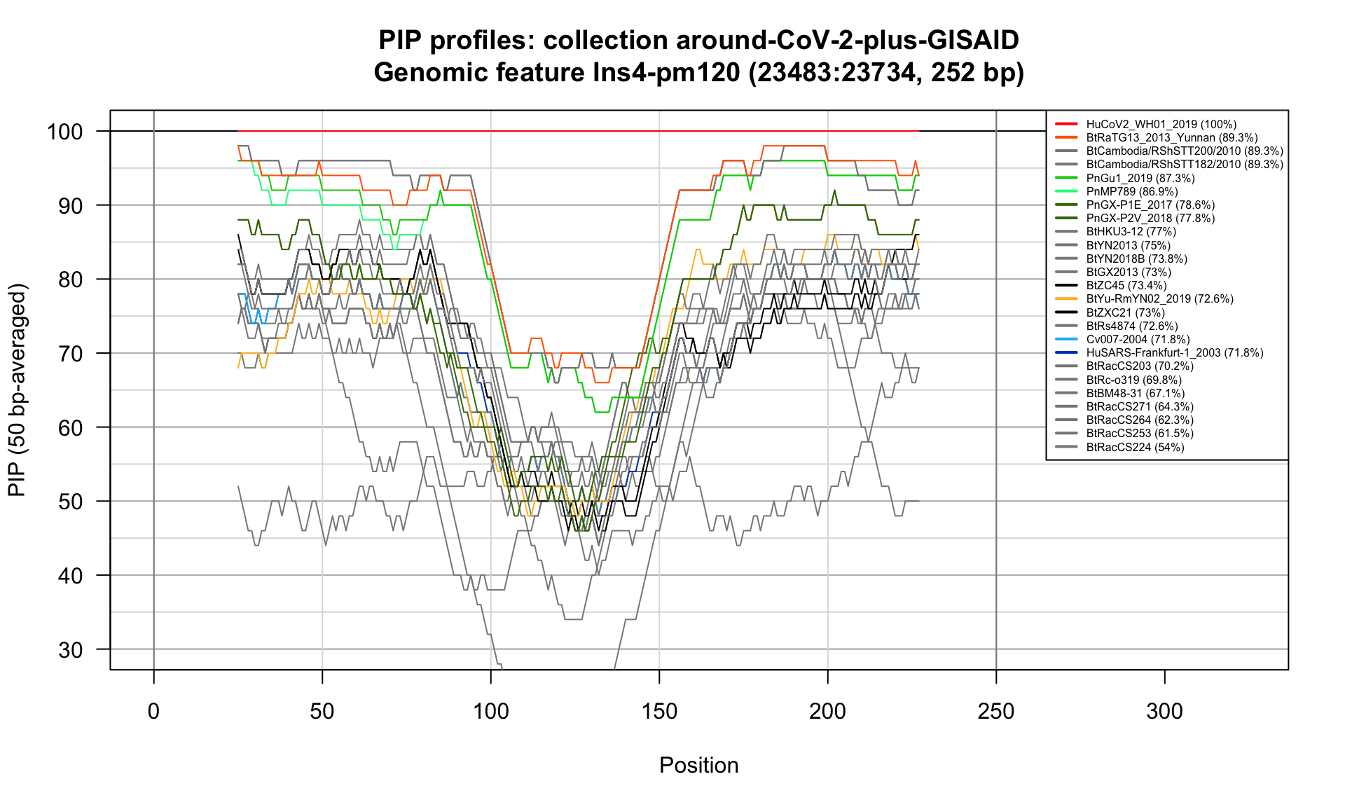
Feature-specific Percent Identical Positions (PIP) profiles.
Ins4-m240 (23363-23614; 252bp)
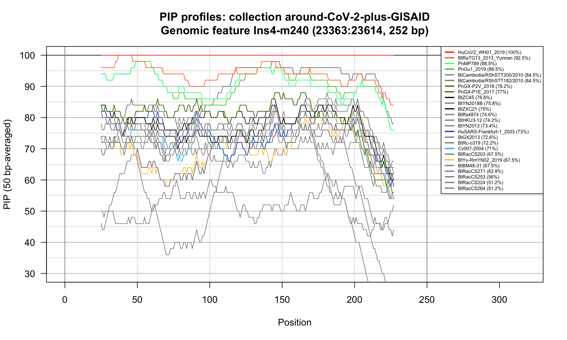
Feature-specific Percent Identical Positions (PIP) profiles.
Recomb-Xiao (22871-23092; 222bp)
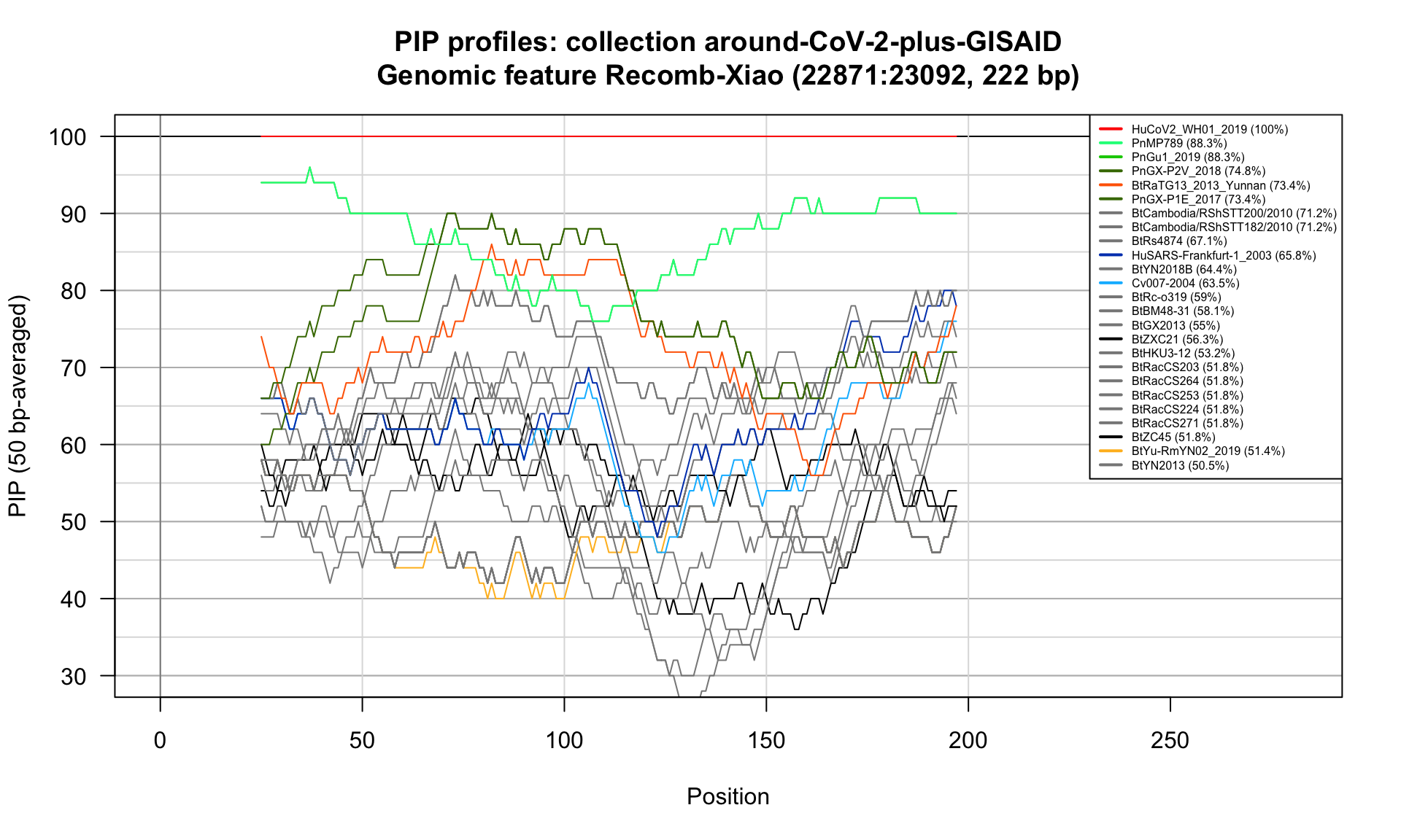
Feature-specific Percent Identical Positions (PIP) profiles.
Recomb-reg-1 (2900-3800; 901bp)
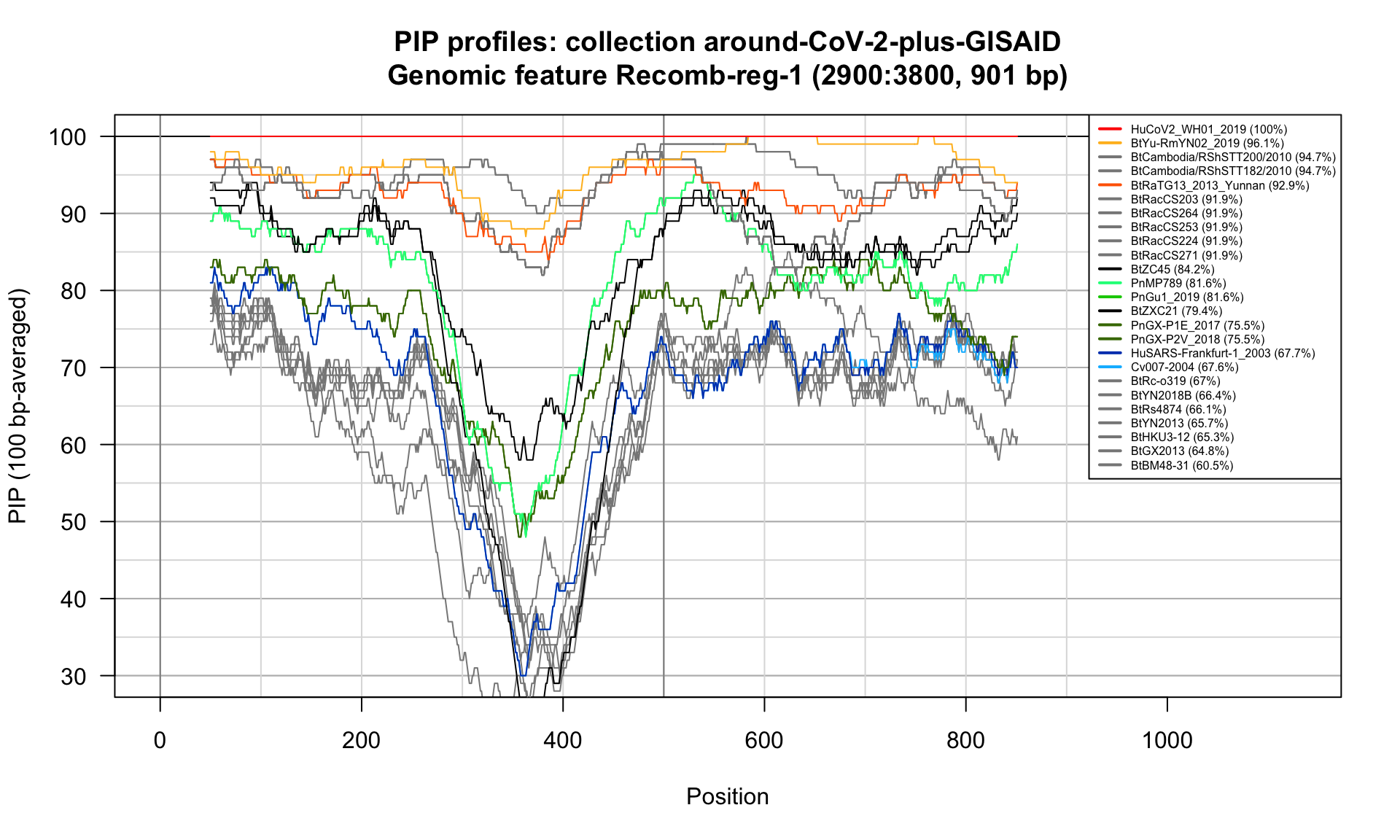
Feature-specific Percent Identical Positions (PIP) profiles.
Recomb-reg-2 (21000-24000; 3001bp)
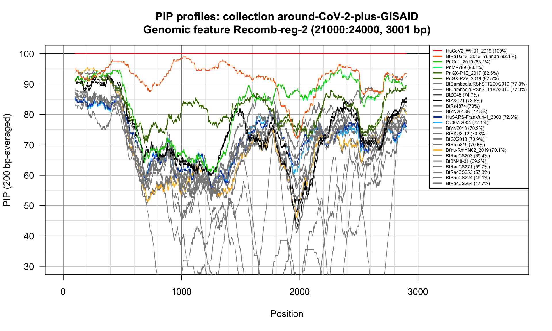
Feature-specific Percent Identical Positions (PIP) profiles.
Recomb-reg-3 (27500-28550; 1051bp)
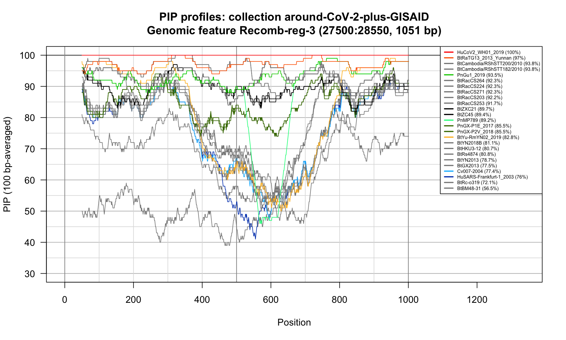
Feature-specific Percent Identical Positions (PIP) profiles.
Recomb-RBD (22700-23200; 501bp)
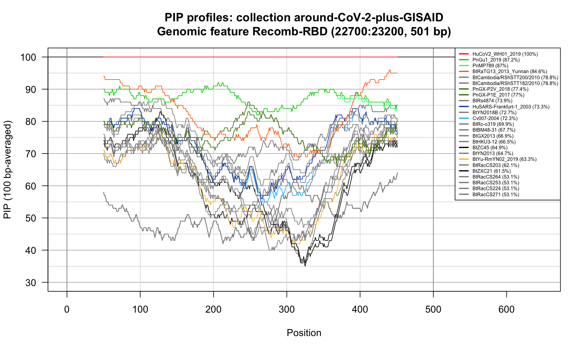
Feature-specific Percent Identical Positions (PIP) profiles.
CDS-S (21563-25384; 3822bp)
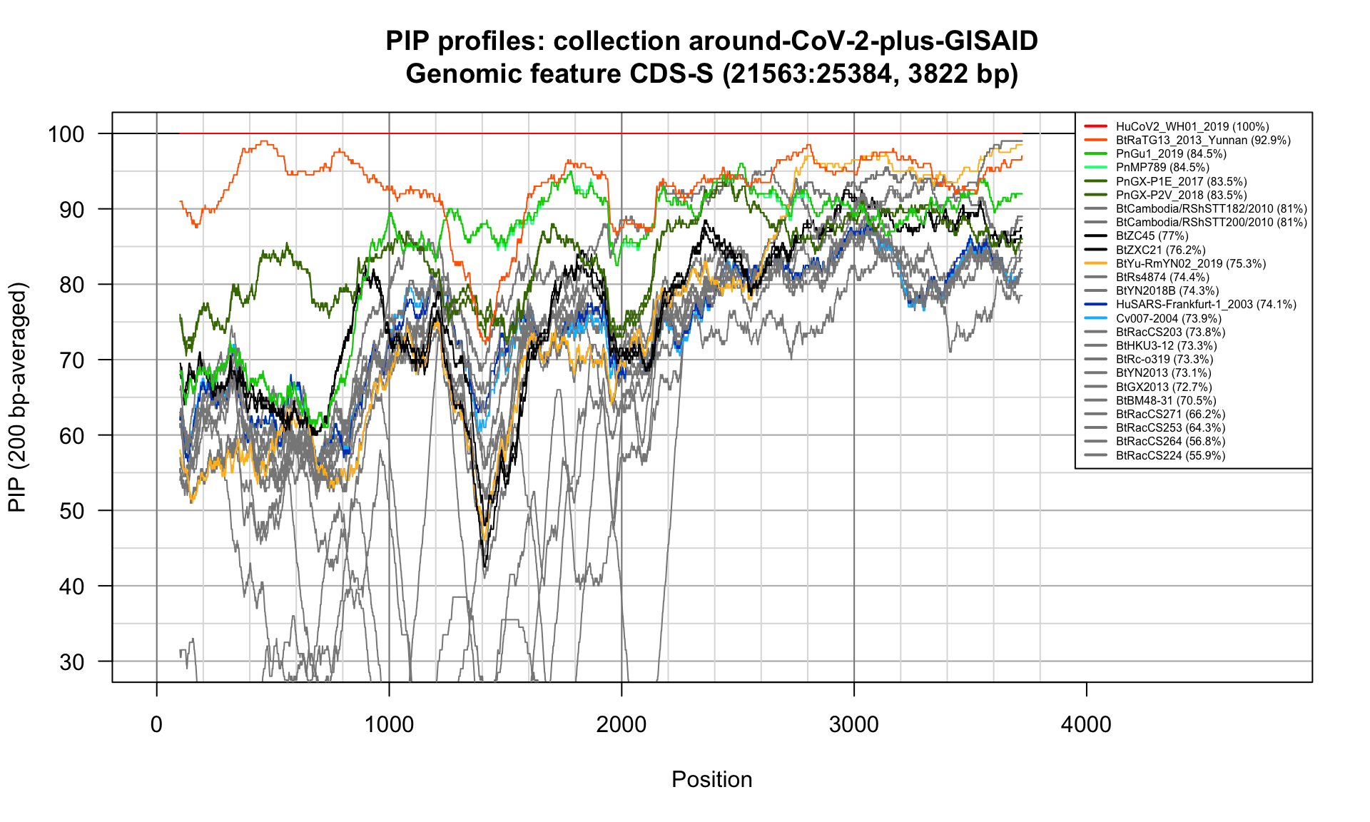
Feature-specific Percent Identical Positions (PIP) profiles.
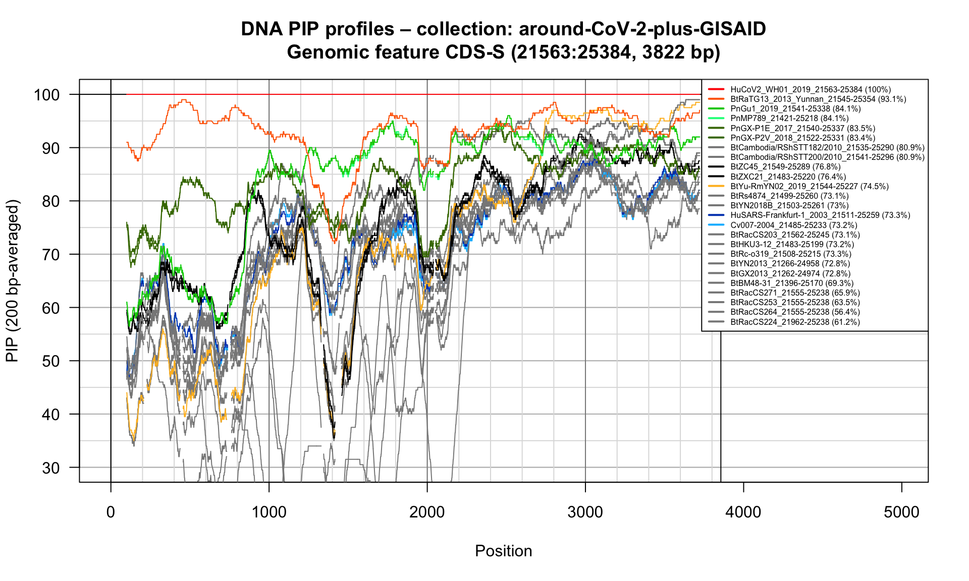
Feature-specific Percent Identical Positions (PIP) profiles.
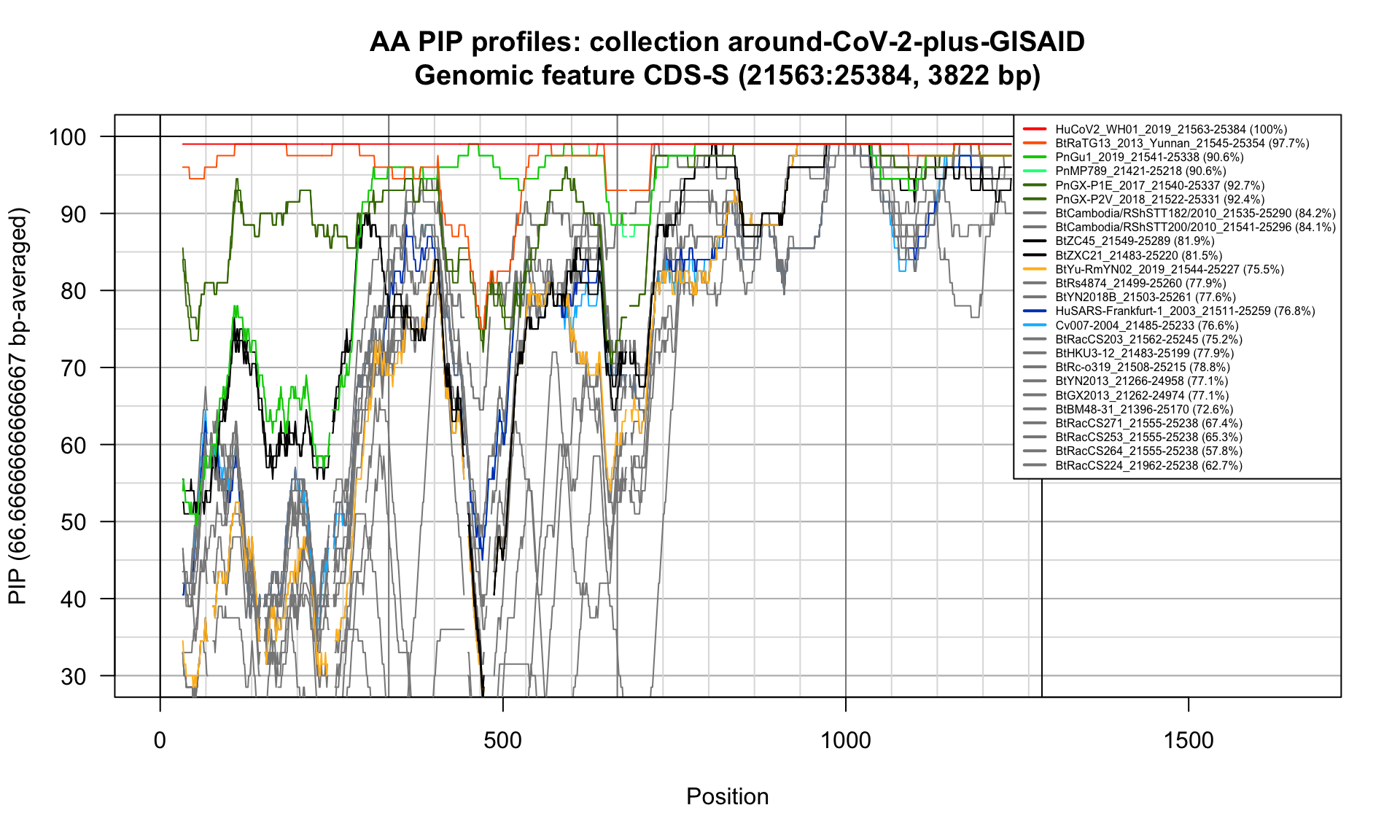
Feature-specific Percent Identical Positions (PIP) profiles.
CDS-ORF3a (25393-26220; 828bp)
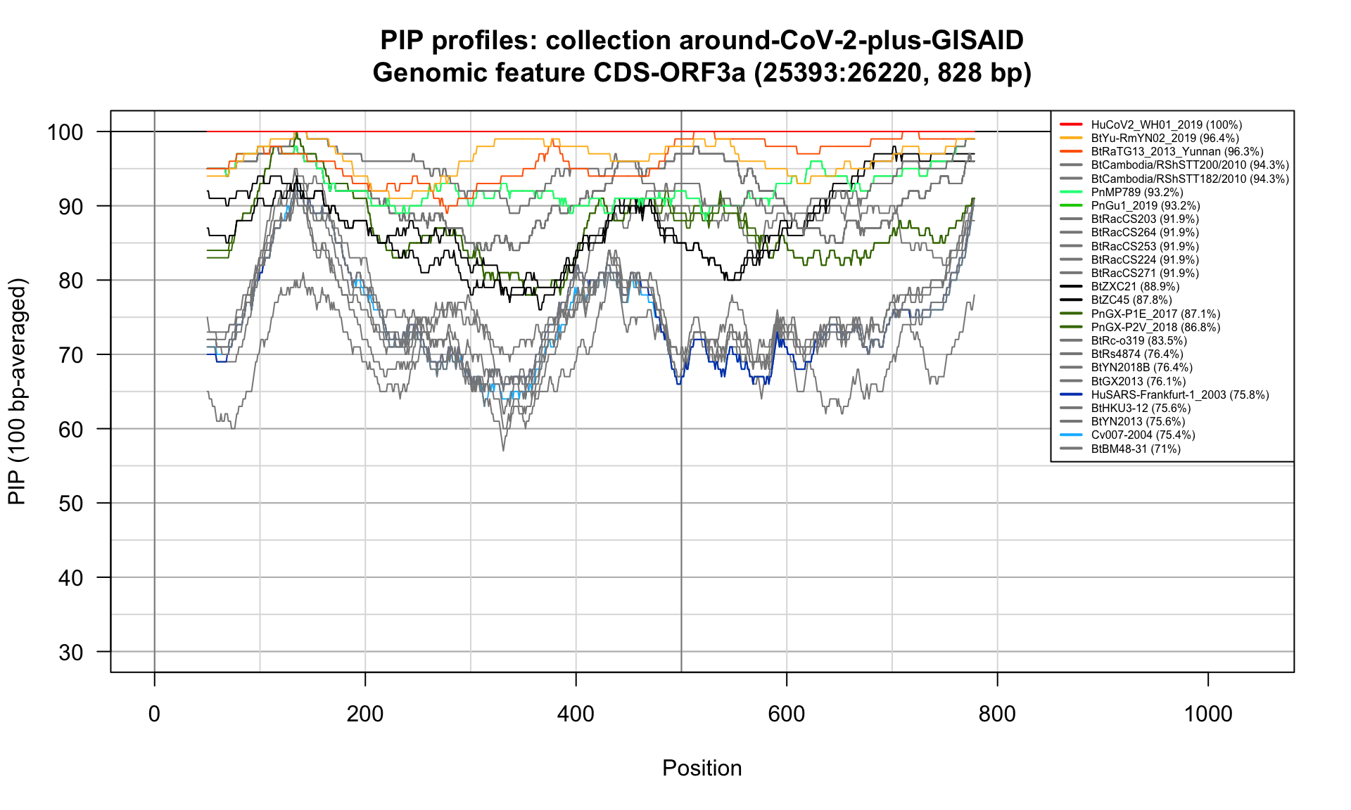
Feature-specific Percent Identical Positions (PIP) profiles.
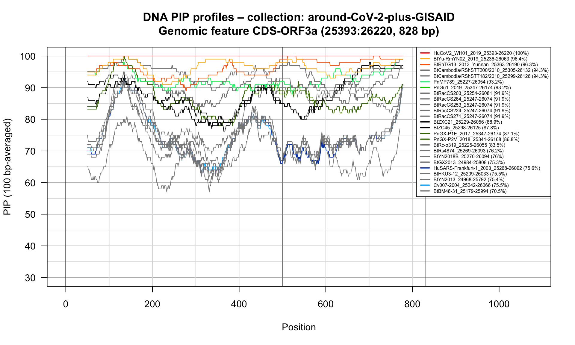
Feature-specific Percent Identical Positions (PIP) profiles.
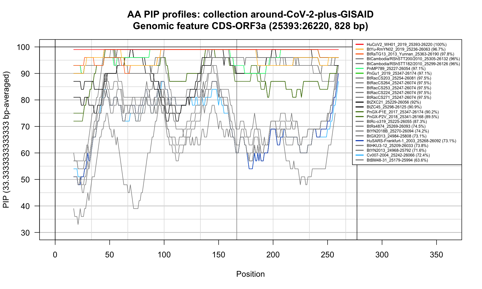
Feature-specific Percent Identical Positions (PIP) profiles.
CDS-E (26245-26472; 228bp)
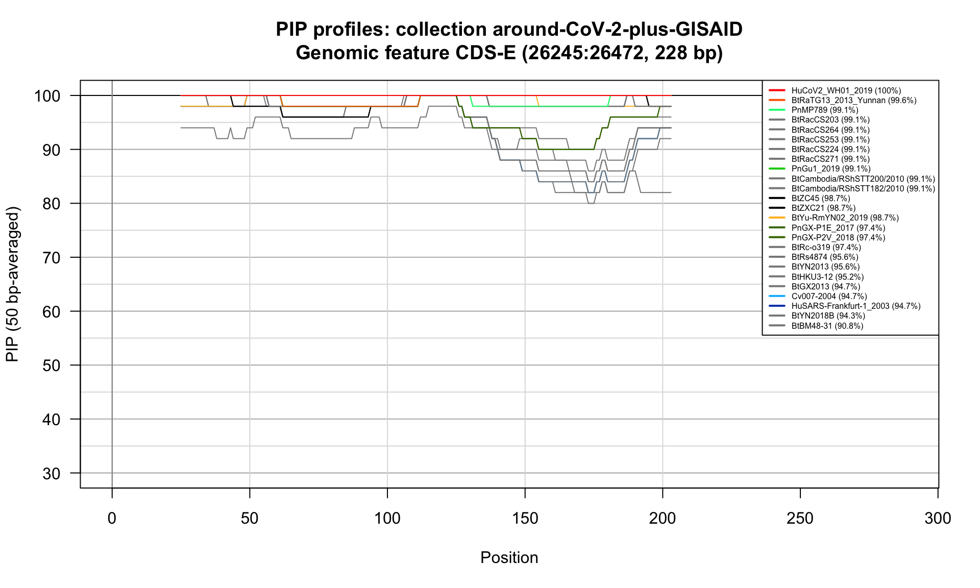
Feature-specific Percent Identical Positions (PIP) profiles.
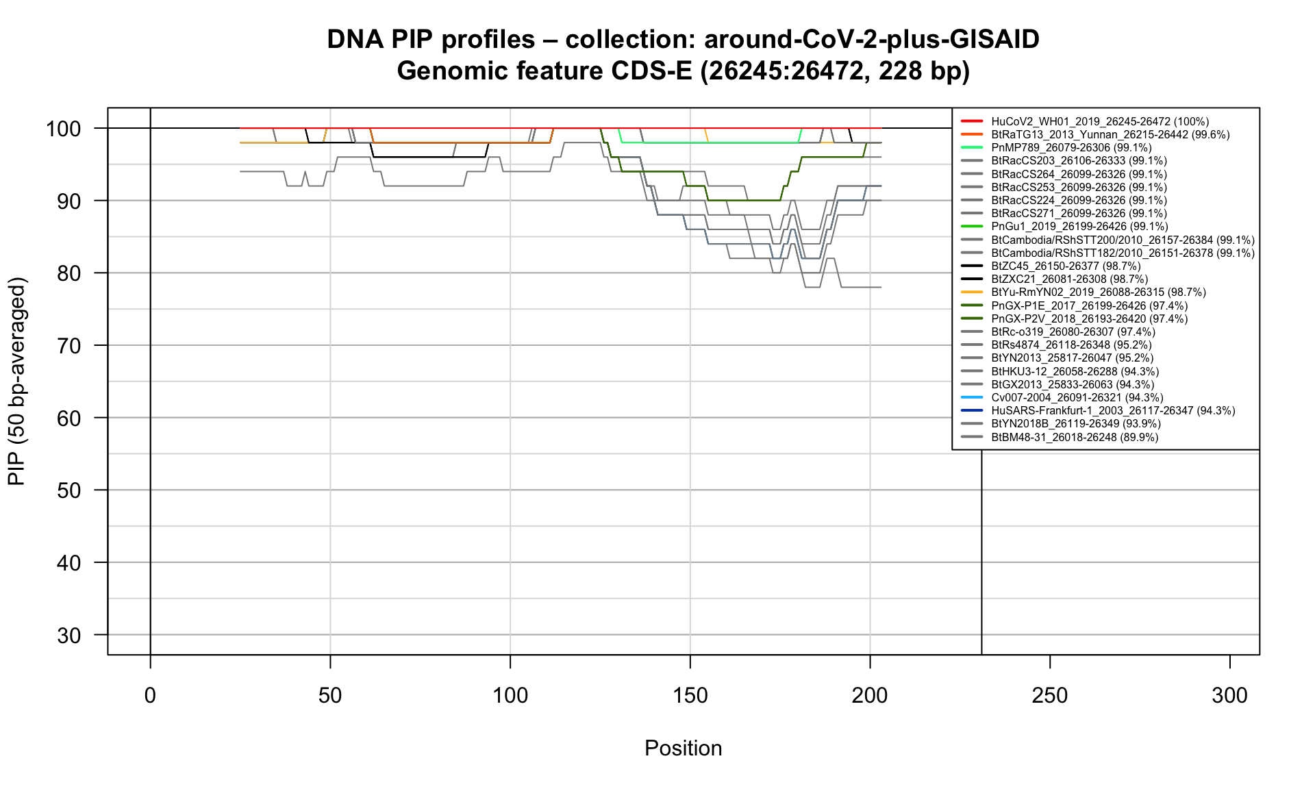
Feature-specific Percent Identical Positions (PIP) profiles.
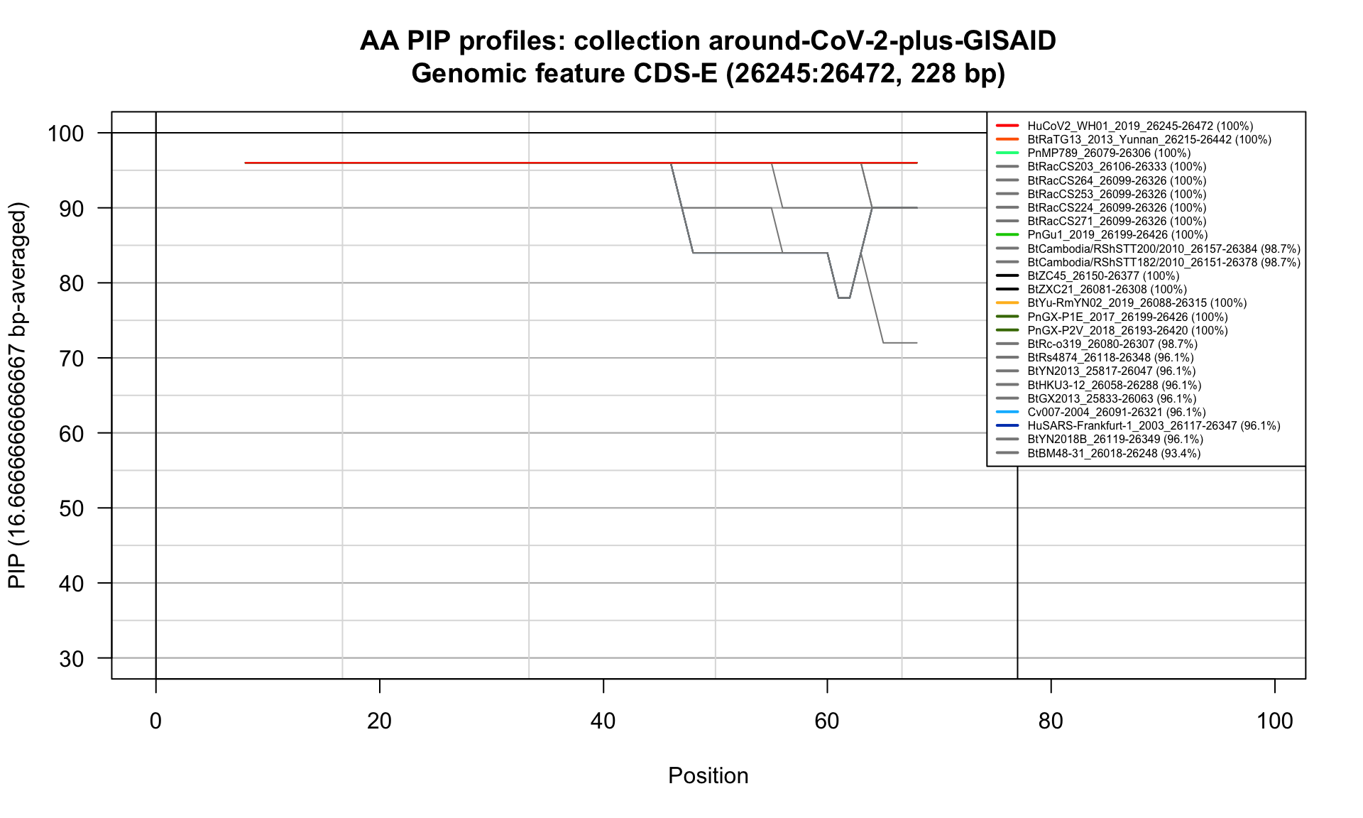
Feature-specific Percent Identical Positions (PIP) profiles.
CDS-M (26523-27191; 669bp)
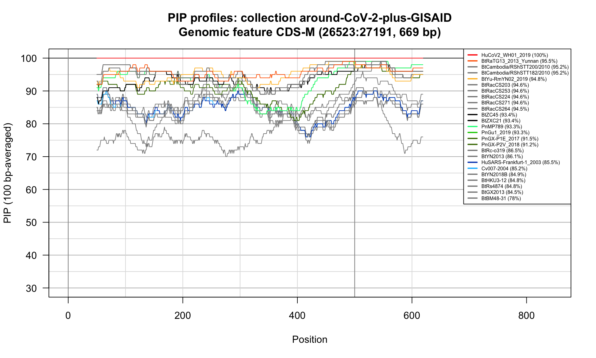
Feature-specific Percent Identical Positions (PIP) profiles.
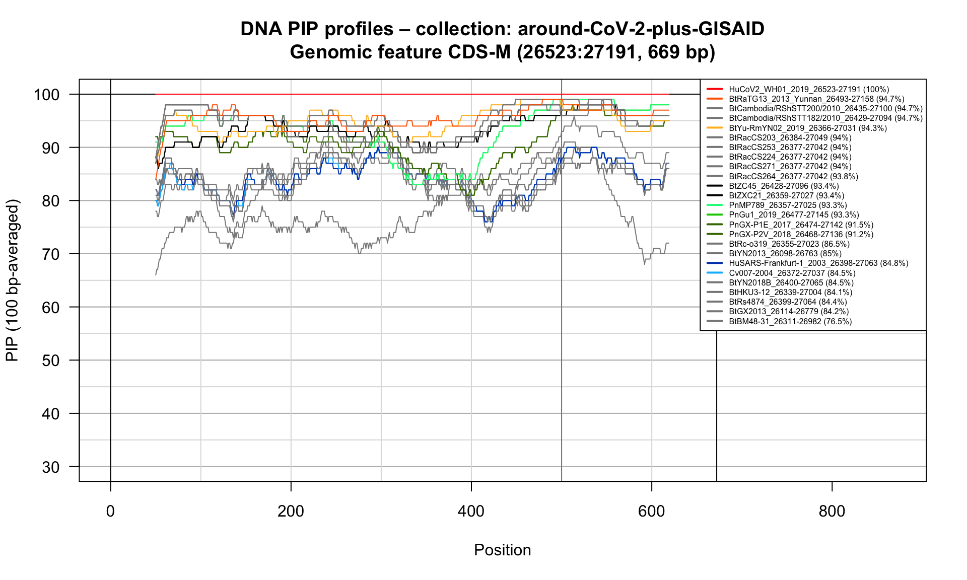
Feature-specific Percent Identical Positions (PIP) profiles.
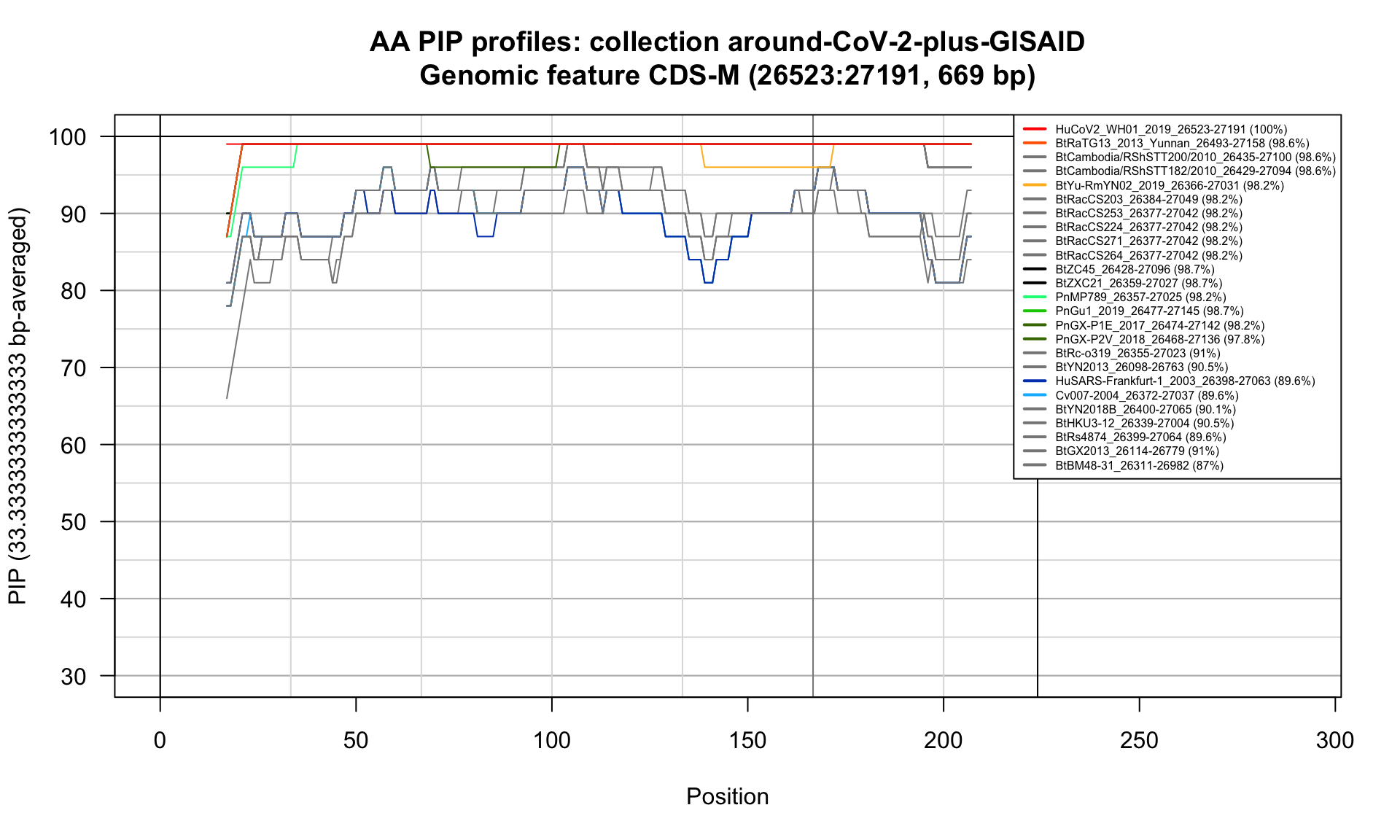
Feature-specific Percent Identical Positions (PIP) profiles.
CDS-ORF6 (27202-27387; 186bp)
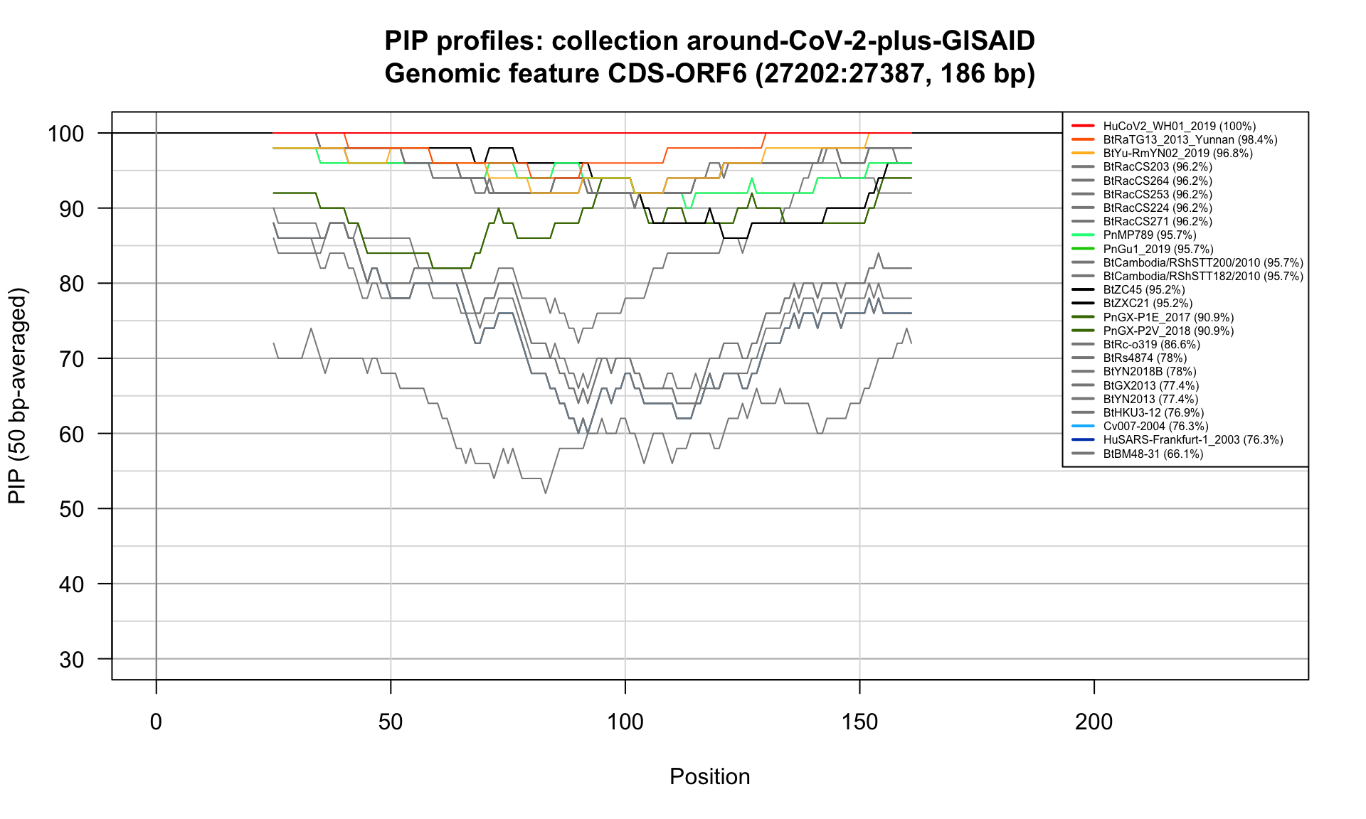
Feature-specific Percent Identical Positions (PIP) profiles.
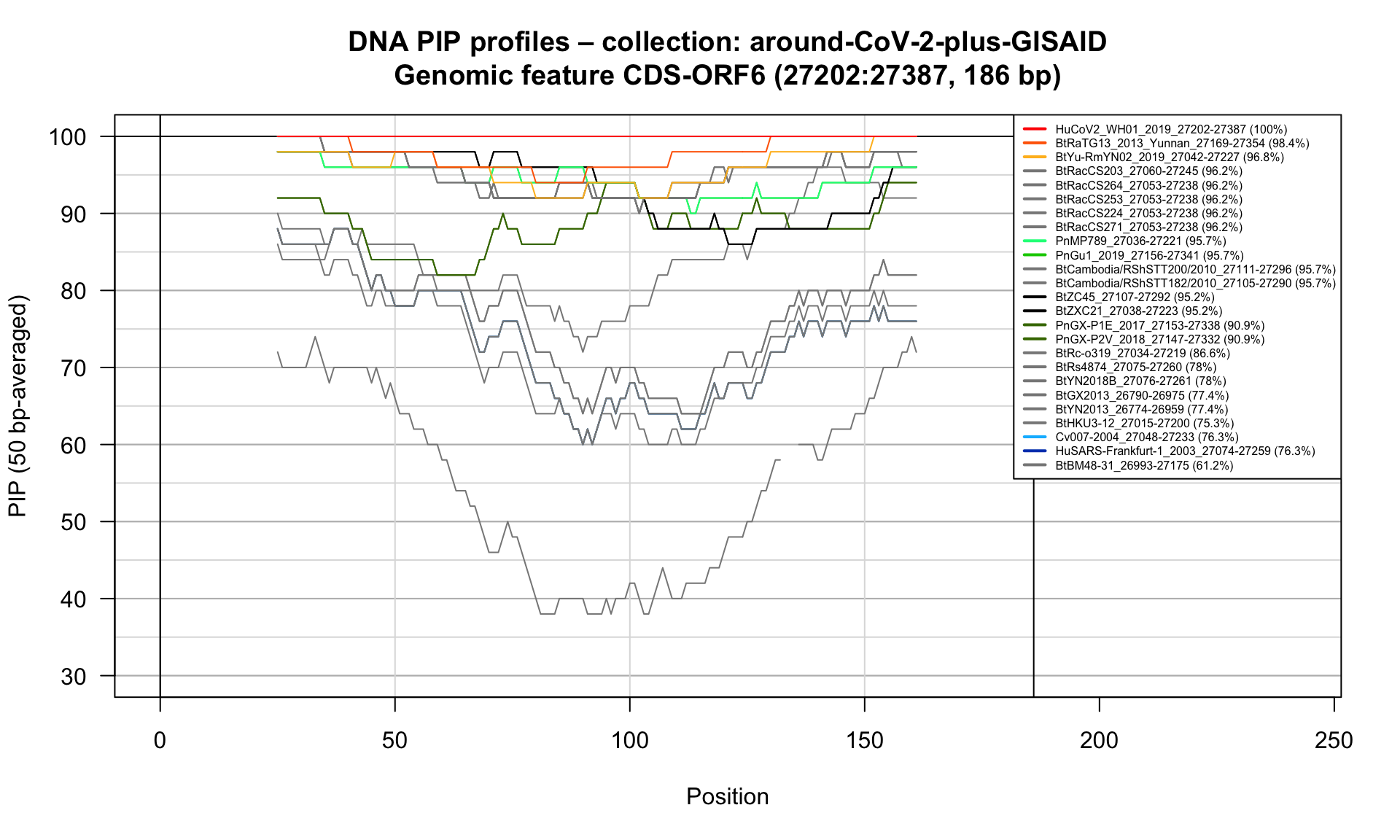
Feature-specific Percent Identical Positions (PIP) profiles.
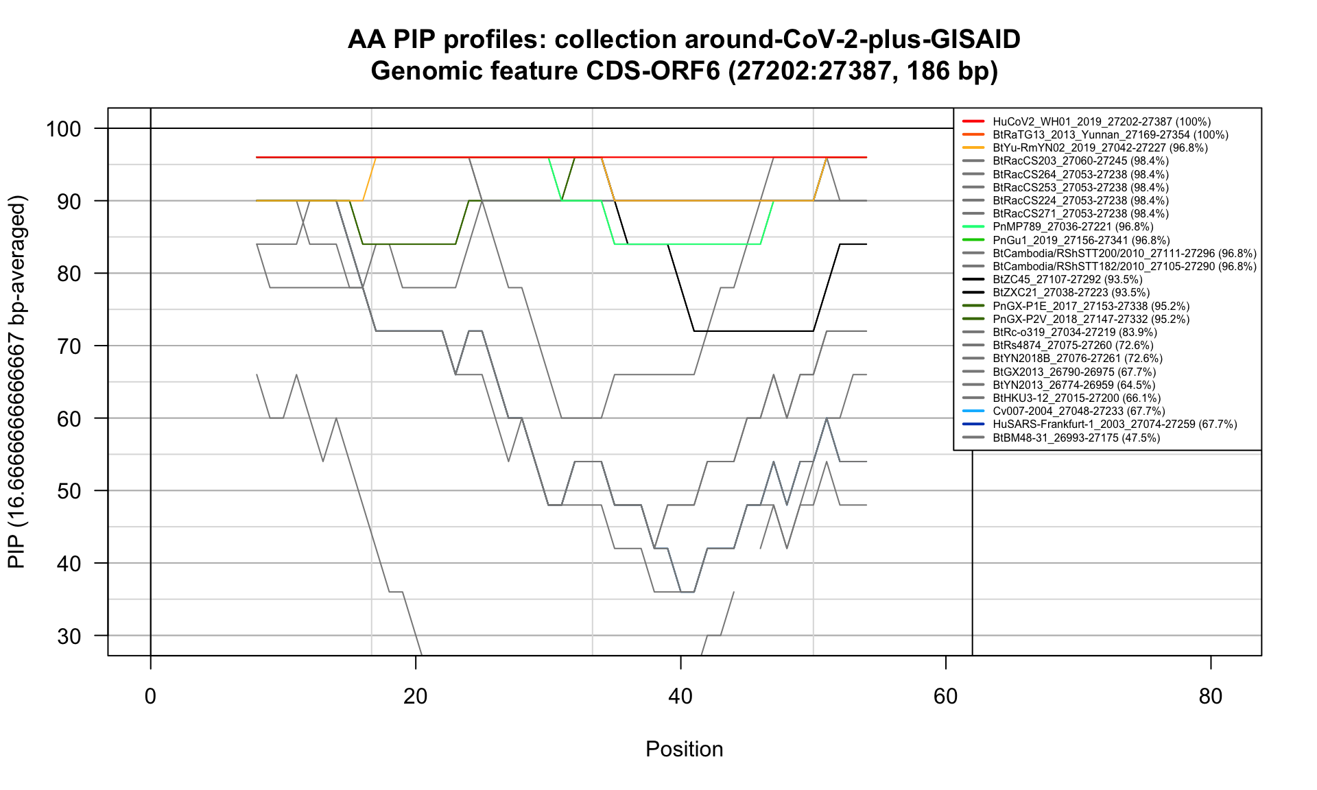
Feature-specific Percent Identical Positions (PIP) profiles.
CDS-ORF7a (27394-27759; 366bp)
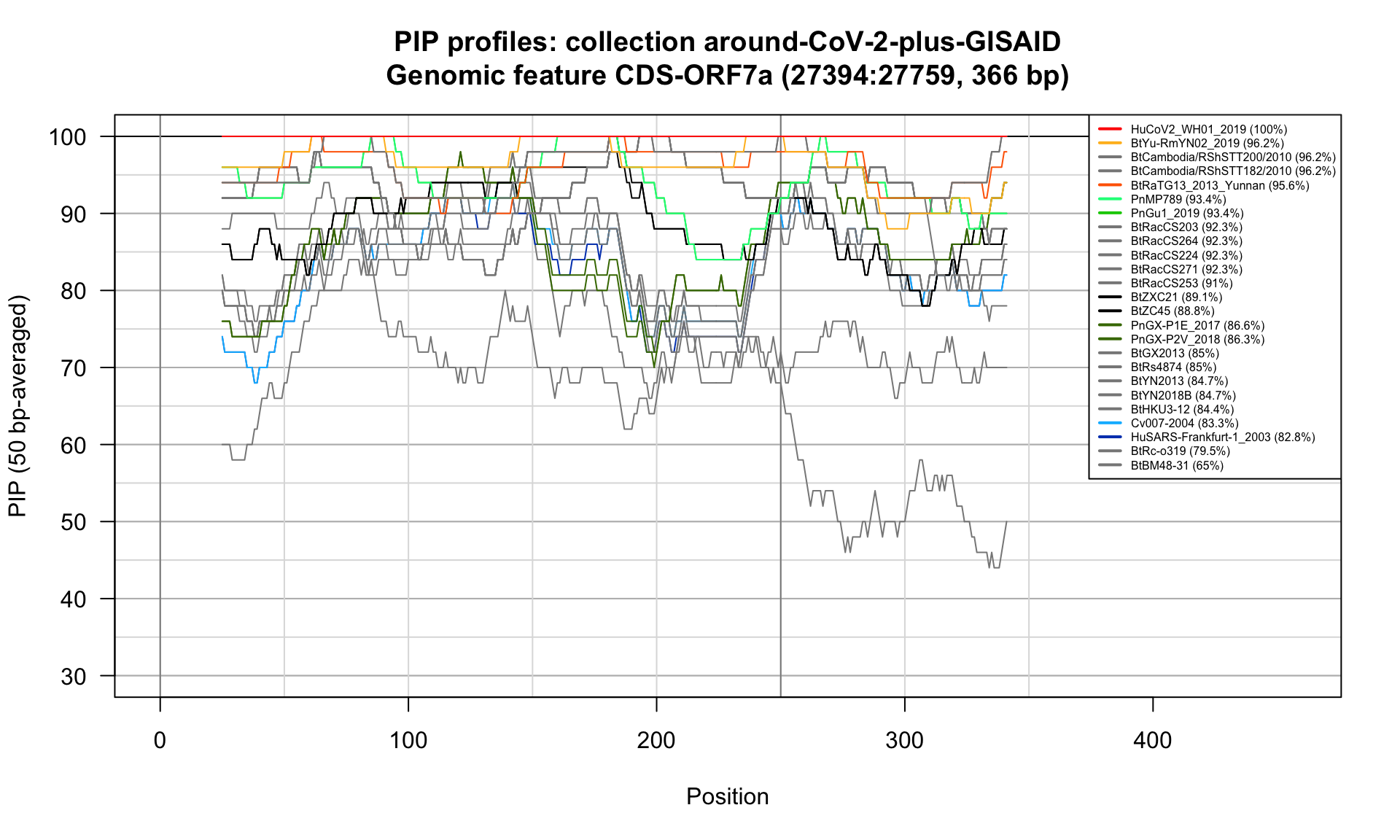
Feature-specific Percent Identical Positions (PIP) profiles.
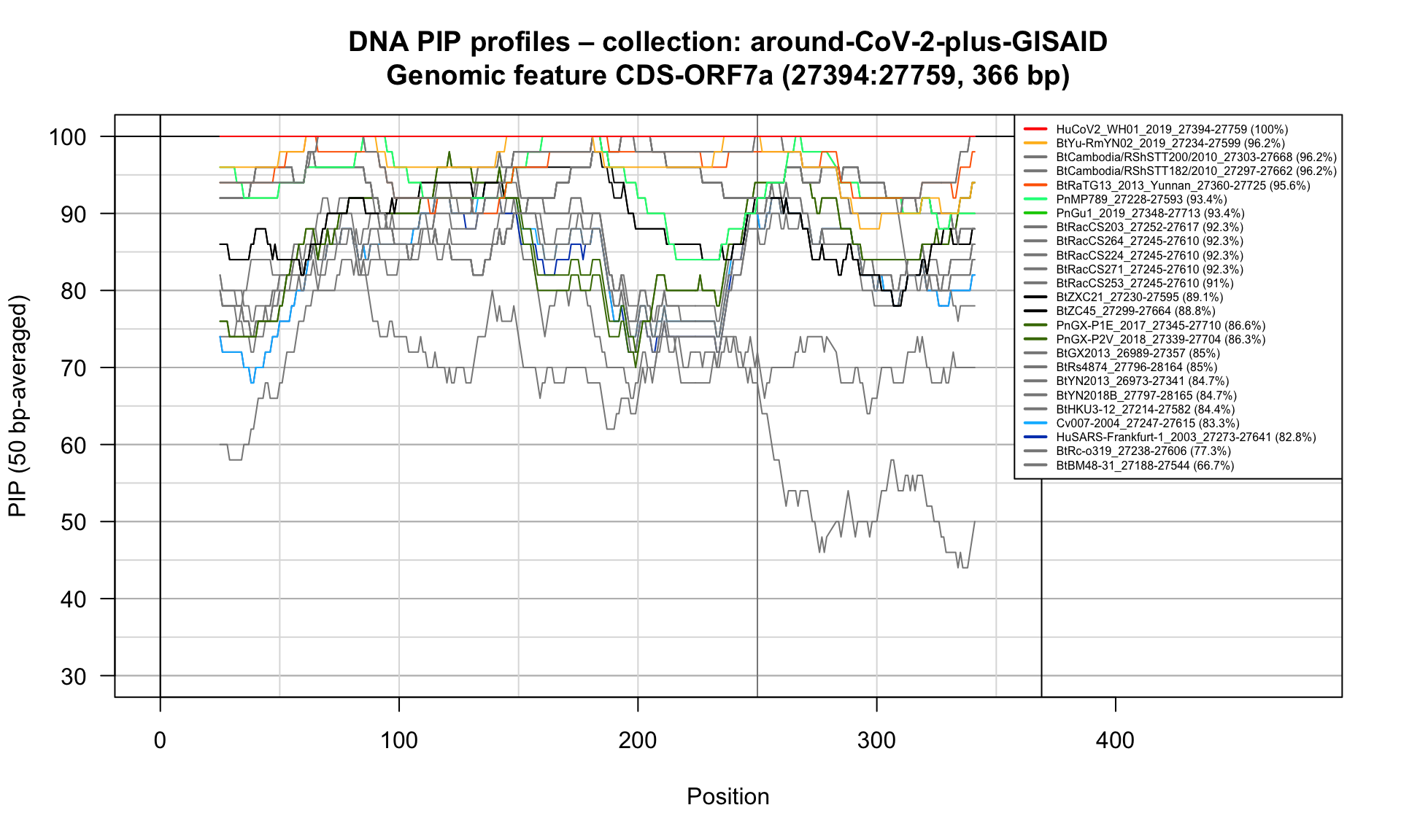
Feature-specific Percent Identical Positions (PIP) profiles.
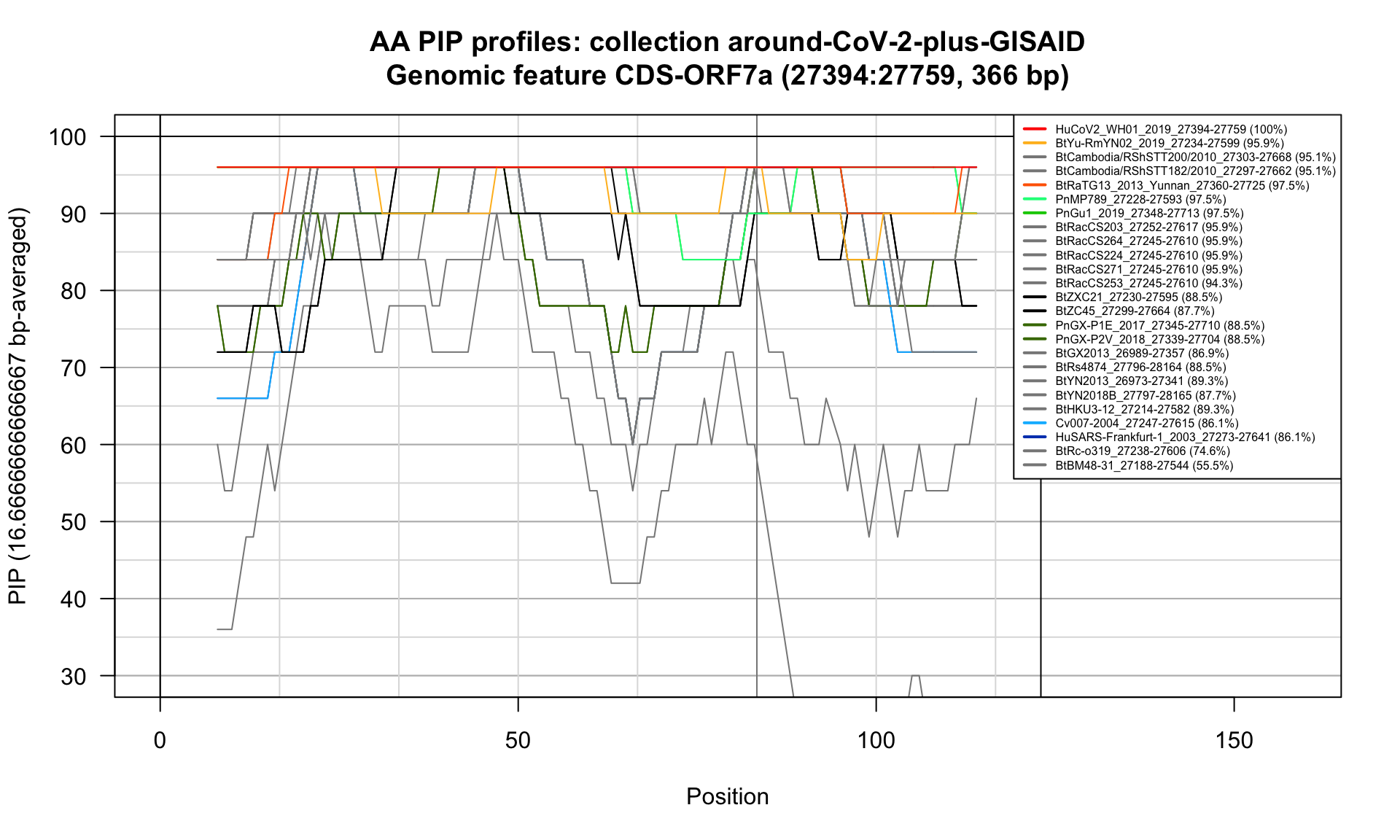
Feature-specific Percent Identical Positions (PIP) profiles.
CDS-ORF8 (27894-28259; 366bp)
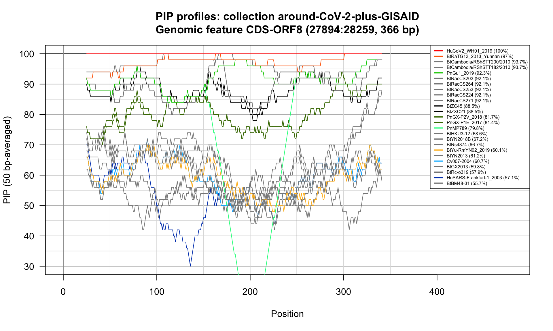
Feature-specific Percent Identical Positions (PIP) profiles.
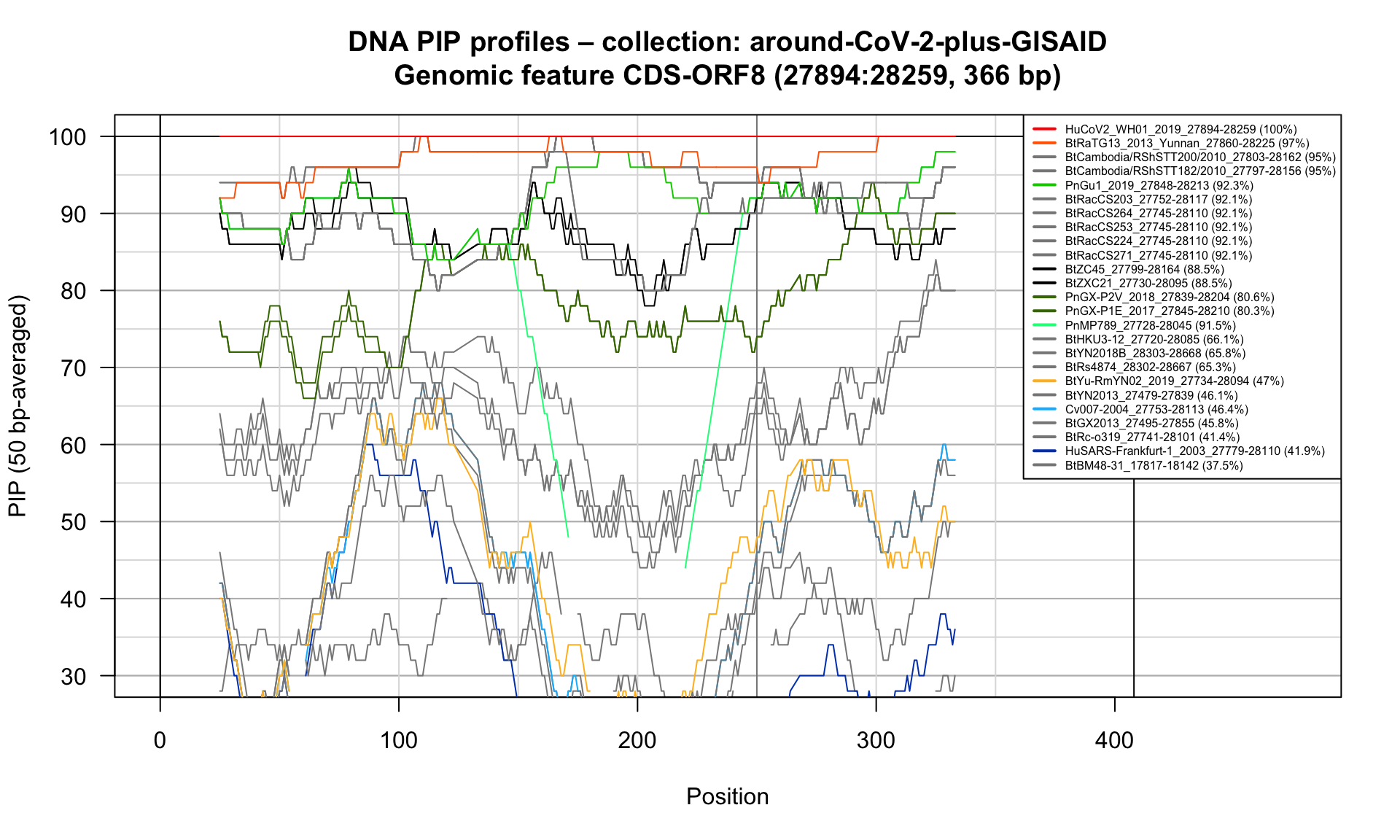
Feature-specific Percent Identical Positions (PIP) profiles.
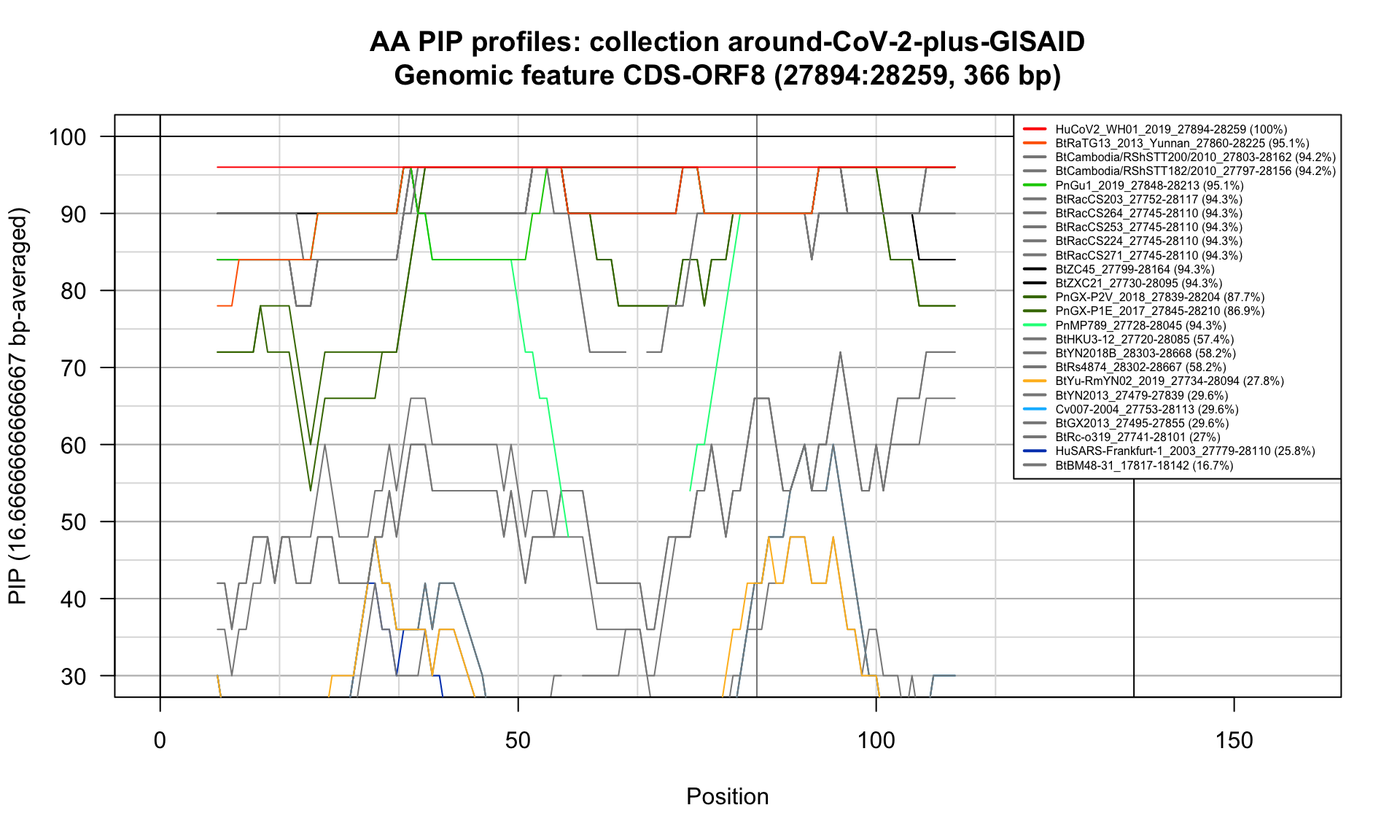
Feature-specific Percent Identical Positions (PIP) profiles.
CDS-N (28274-29533; 1260bp)
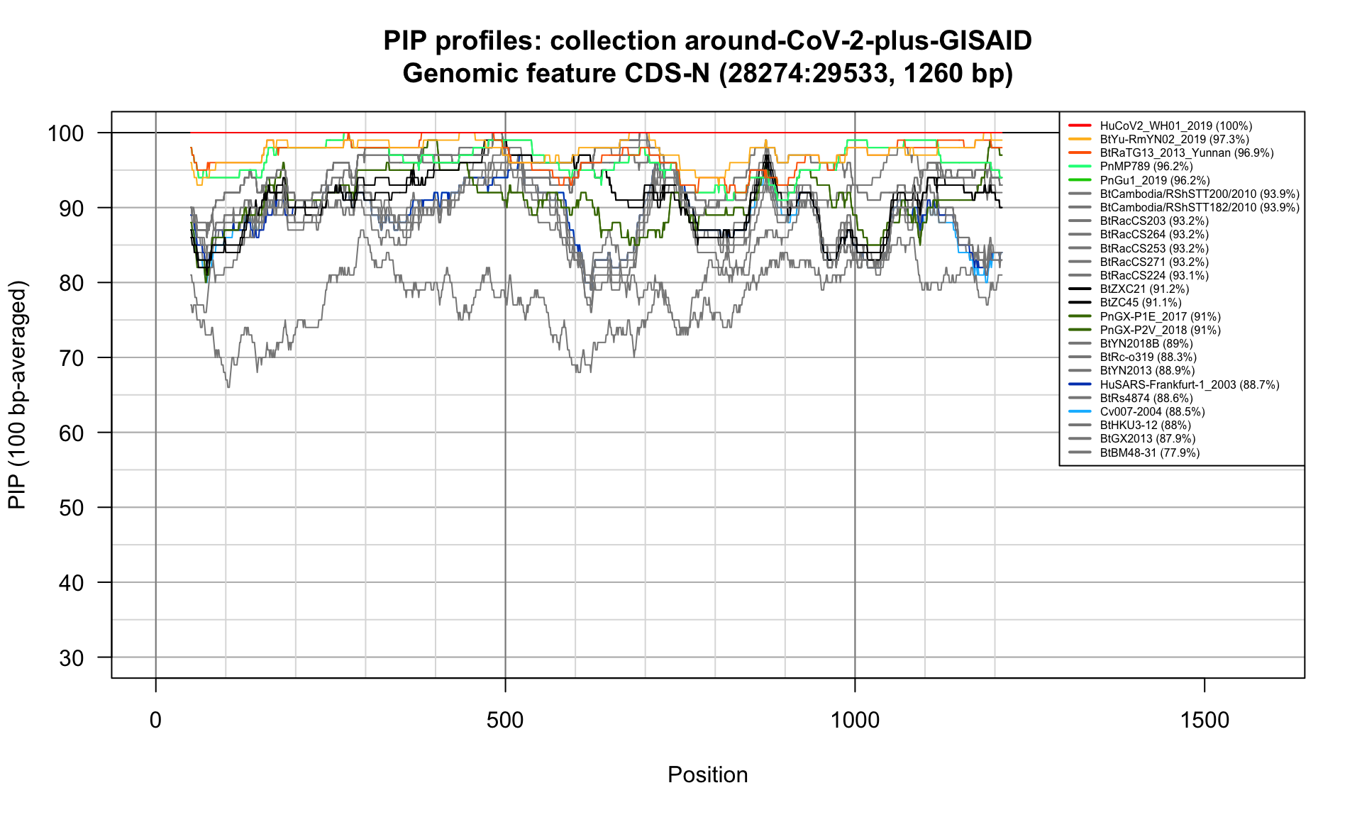
Feature-specific Percent Identical Positions (PIP) profiles.
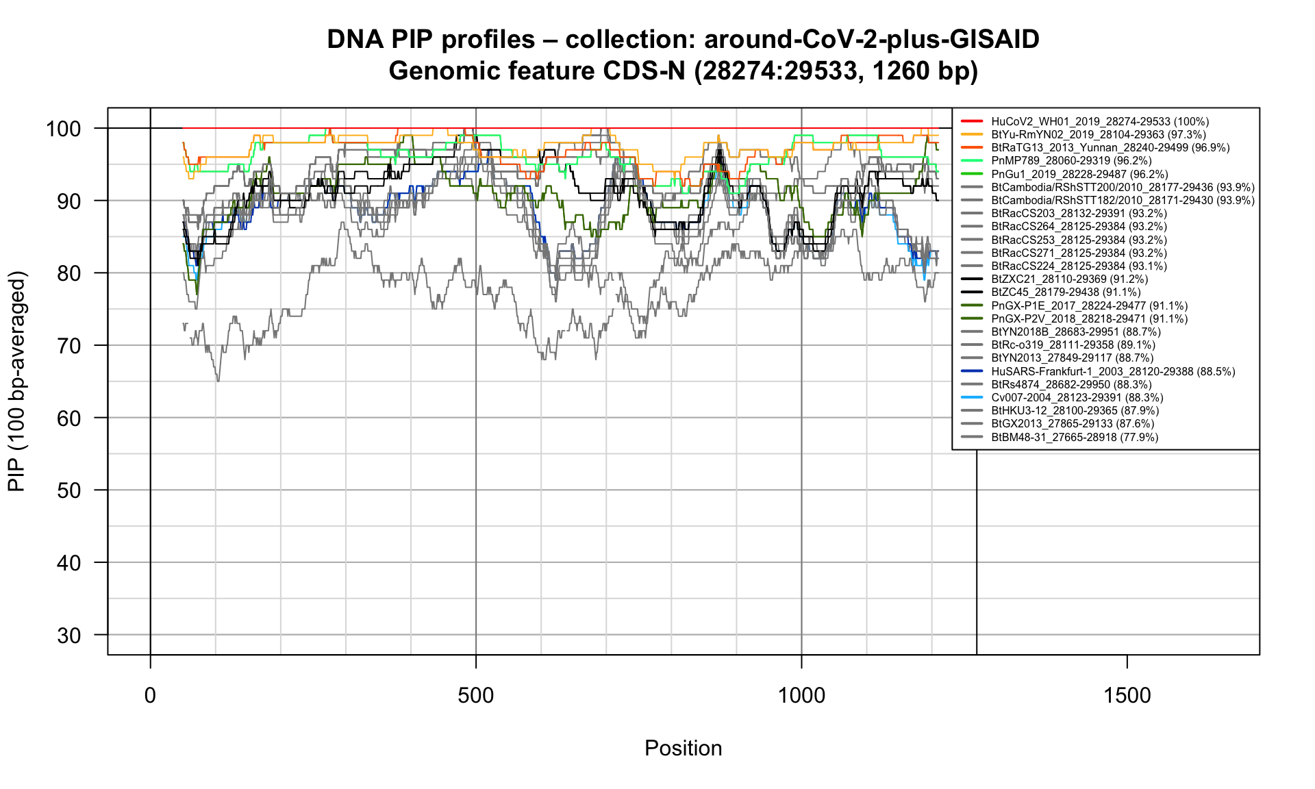
Feature-specific Percent Identical Positions (PIP) profiles.
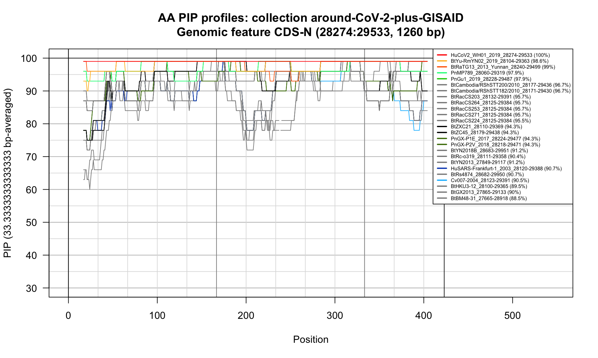
Feature-specific Percent Identical Positions (PIP) profiles.
CDS-ORF10 (29558-29674; 117bp)
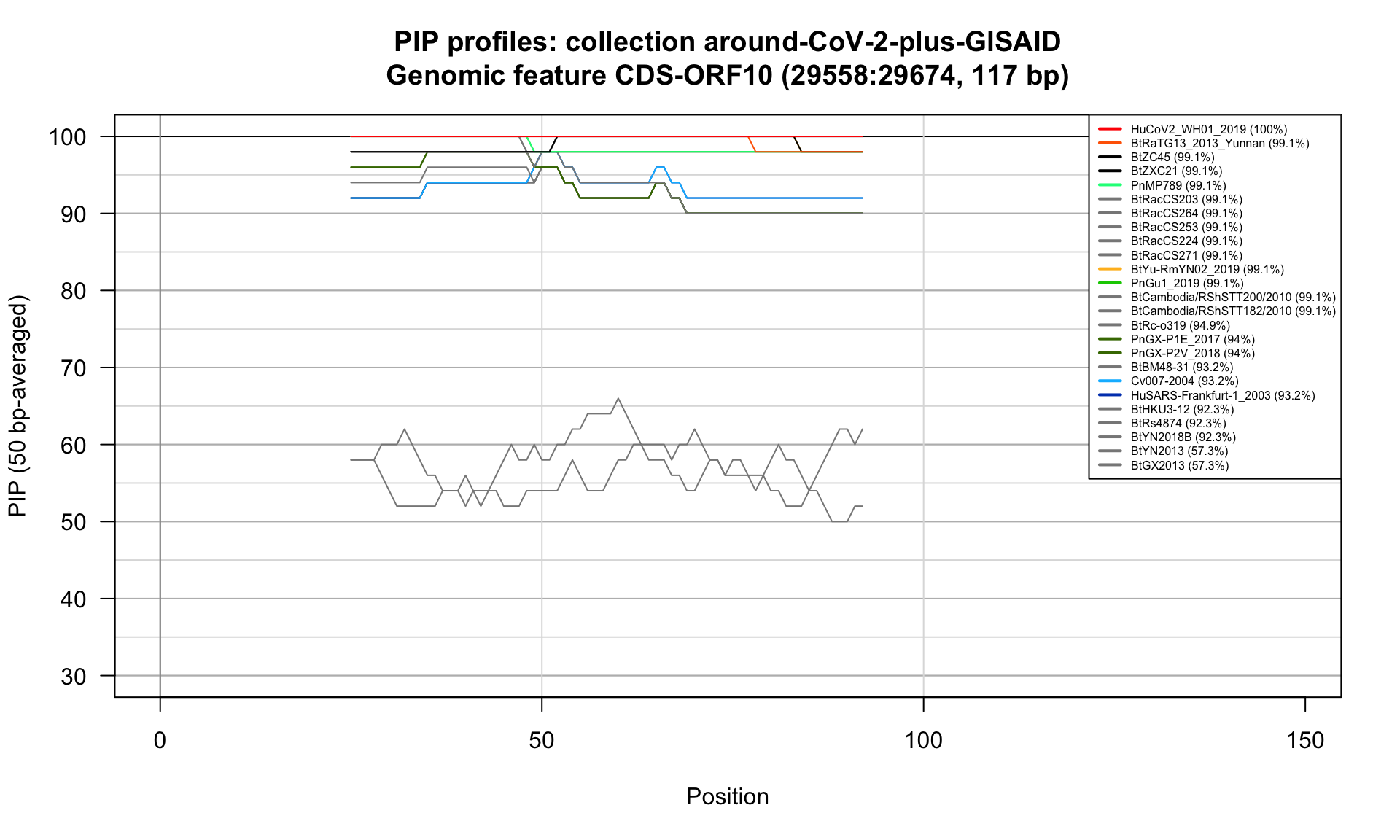
Feature-specific Percent Identical Positions (PIP) profiles.
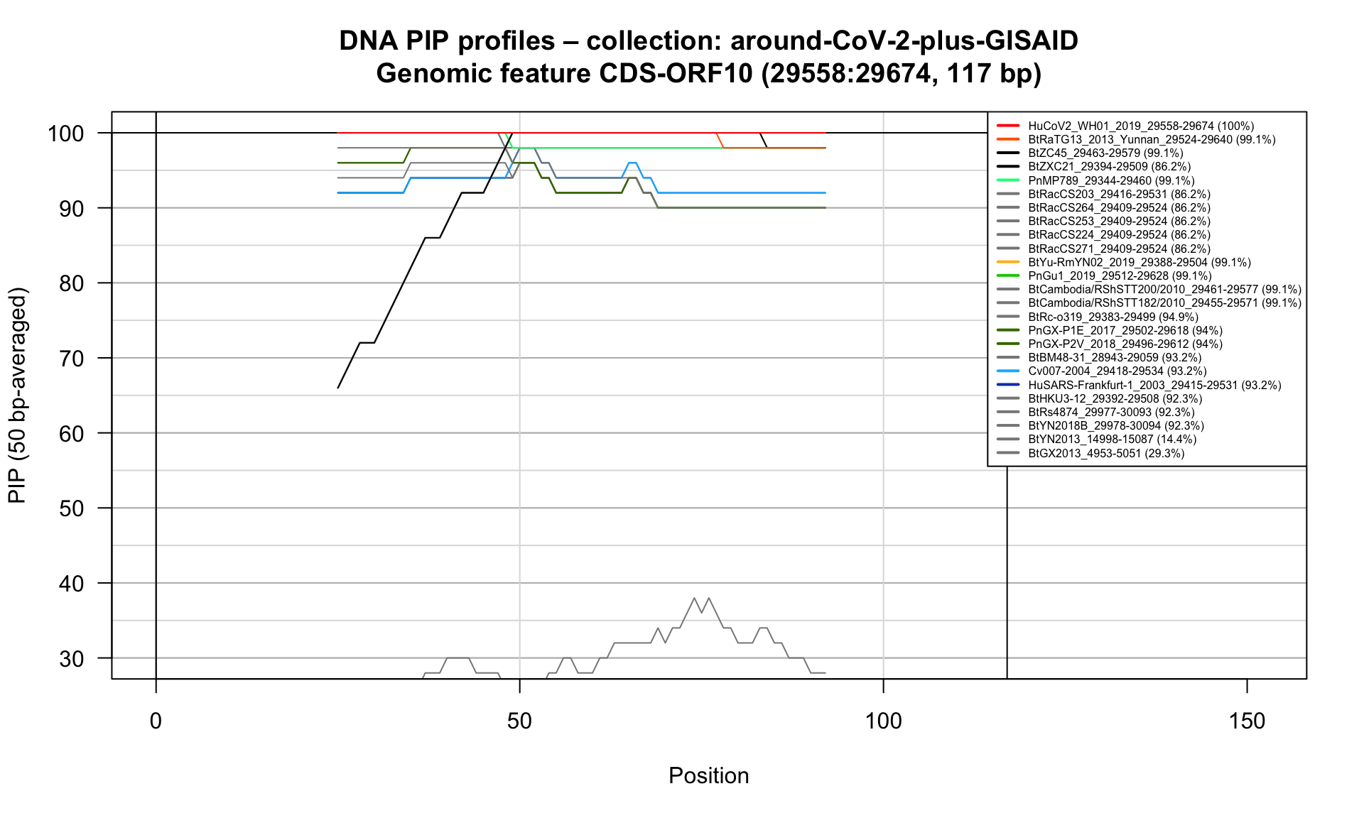
Feature-specific Percent Identical Positions (PIP) profiles.
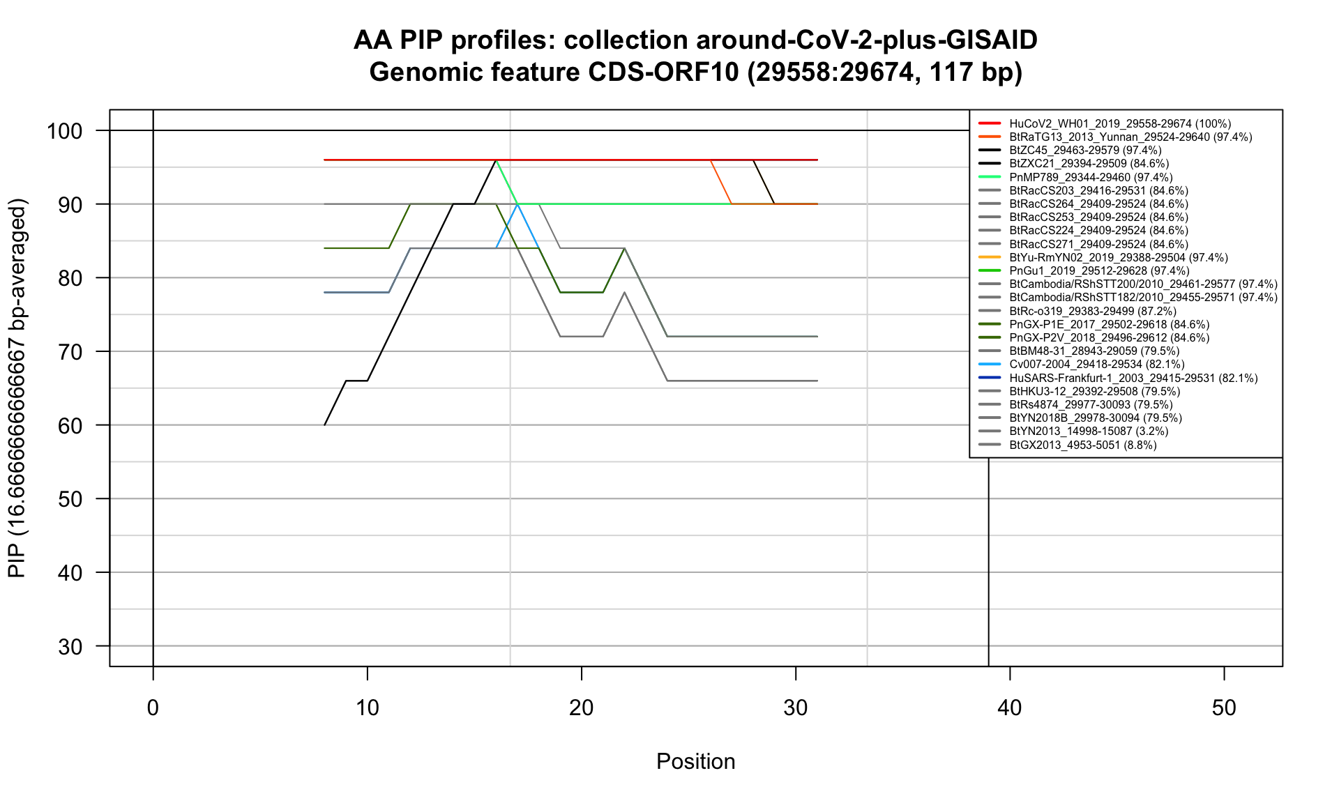
Feature-specific Percent Identical Positions (PIP) profiles.
CDS-ORF1ab (266-21555; 21290bp)
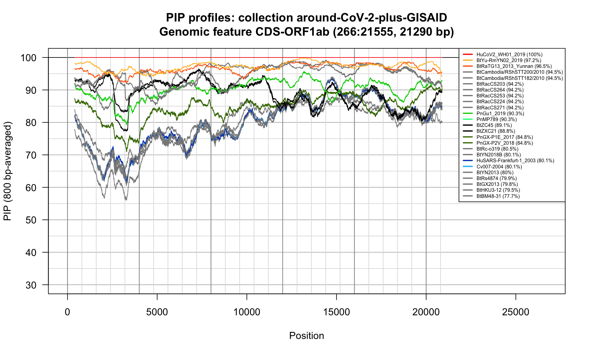
Feature-specific Percent Identical Positions (PIP) profiles.

Feature-specific Percent Identical Positions (PIP) profiles.

Feature-specific Percent Identical Positions (PIP) profiles.
Output files
| Dir | |
|---|---|
| main | .. |
| R | ../scripts/R |
| seqdata | ../data |
| results | ../results |
| images | ../memory_images |
| sequences | ../data/GISAID_genomes |
| Sun_2020 | ../results/Sun_2020_around-CoV-2-plus-GISAID |
| S1 | ../results/S1_around-CoV-2-plus-GISAID |
| RBD | ../results/RBD_around-CoV-2-plus-GISAID |
| S2 | ../results/S2_around-CoV-2-plus-GISAID |
| Ins1.pm120 | ../results/Ins1-pm120_around-CoV-2-plus-GISAID |
| Ins2.pm120 | ../results/Ins2-pm120_around-CoV-2-plus-GISAID |
| Ins3.pm120 | ../results/Ins3-pm120_around-CoV-2-plus-GISAID |
| Ins4.pm120 | ../results/Ins4-pm120_around-CoV-2-plus-GISAID |
| Ins4.m240 | ../results/Ins4-m240_around-CoV-2-plus-GISAID |
| Recomb.Xiao | ../results/Recomb-Xiao_around-CoV-2-plus-GISAID |
| Recomb.reg.1 | ../results/Recomb-reg-1_around-CoV-2-plus-GISAID |
| Recomb.reg.2 | ../results/Recomb-reg-2_around-CoV-2-plus-GISAID |
| Recomb.reg.3 | ../results/Recomb-reg-3_around-CoV-2-plus-GISAID |
| Recomb.RBD | ../results/Recomb-RBD_around-CoV-2-plus-GISAID |
| CDS.S | ../results/CDS-S_around-CoV-2-plus-GISAID |
| CDS.ORF3a | ../results/CDS-ORF3a_around-CoV-2-plus-GISAID |
| CDS.E | ../results/CDS-E_around-CoV-2-plus-GISAID |
| CDS.M | ../results/CDS-M_around-CoV-2-plus-GISAID |
| CDS.ORF6 | ../results/CDS-ORF6_around-CoV-2-plus-GISAID |
| CDS.ORF7a | ../results/CDS-ORF7a_around-CoV-2-plus-GISAID |
| CDS.ORF8 | ../results/CDS-ORF8_around-CoV-2-plus-GISAID |
| CDS.N | ../results/CDS-N_around-CoV-2-plus-GISAID |
| CDS.ORF10 | ../results/CDS-ORF10_around-CoV-2-plus-GISAID |
| CDS.ORF1ab | ../results/CDS-ORF1ab_around-CoV-2-plus-GISAID |
| After.ORF1ab | ../results/After-ORF1ab_around-CoV-2-plus-GISAID |
outfileTable <- data.frame(path = as.vector(outfiles))
outfileTable$basename <- basename(as.vector(outfileTable$path))
outfileTable$dir <- dirname(as.vector(outfileTable$path))
outfileTable$link <- paste0(
  "[", outfileTable$basename, "](", outfileTable$path, ")"
)

kable(outfileTable[, c("dir", "link")],
      col.names = c("dir", "file"),
caption = "Output files")Memory image
We store the result ina memory image, in oder to be able reloading it to plot PIP profiles with different parameters.
Session info
R version 4.0.2 (2020-06-22)
Platform: x86_64-apple-darwin17.0 (64-bit)
Running under: macOS Mojave 10.14.6

Matrix products: default
BLAS:   /Library/Frameworks/R.framework/Versions/4.0/Resources/lib/libRblas.dylib
LAPACK: /Library/Frameworks/R.framework/Versions/4.0/Resources/lib/libRlapack.dylib

locale:
[1] en_US.UTF-8/en_US.UTF-8/en_US.UTF-8/C/en_US.UTF-8/en_US.UTF-8

attached base packages:
[1] stats4    parallel  stats     graphics  grDevices utils     datasets  methods   base

other attached packages:
[1] DECIPHER_2.16.1     RSQLite_2.2.1       Biostrings_2.56.0   XVector_0.28.0      IRanges_2.22.2      S4Vectors_0.26.1    BiocGenerics_0.34.0 knitr_1.30

loaded via a namespace (and not attached):
 [1] Rcpp_1.0.5          magrittr_1.5        zlibbioc_1.34.0     bit_4.0.4           rlang_0.4.8         highr_0.8           stringr_1.4.0       blob_1.2.1          tools_4.0.2         xfun_0.19           DBI_1.1.0           htmltools_0.5.0     yaml_2.2.1          bit64_4.0.5
[15] digest_0.6.27 crayon_1.3.4 BiocManager_1.30.10 vctrs_0.3.4 memoise_1.1.0 evaluate_0.14 rmarkdown_2.5 stringi_1.5.3 compiler_4.0.2 