Markov Models part 1: nothing to hide so far. Solutions
Computational biology
Jacques van Helden
2019-12-18
if (!require("gplots")) {
   install.packages("gplots", dependencies = TRUE)
   library(gplots)
   }
if (!require("RColorBrewer")) {
   install.packages("RColorBrewer", dependencies = TRUE)
   library(RColorBrewer)
   }
CpG island length distribution
## Load CpG island coordinates
CpG.coord <- read.delim(file = "results/hg38/hg38_CpG_islands.bed.gz", header = FALSE)

names(CpG.coord) <- c("chr", "start", "end", "id")
## Note: bed convention : the end marks the first position
## **after** the feature, so the length is simply the difference
CpG.coord$length <- CpG.coord$end - CpG.coord$start
genome.size <- 3e+9
## Compute statistics about CpG island lengths
CpG.length.stat <- data.frame(
nb = nrow(CpG.coord),
min = min(CpG.coord$length),
Q1 = quantile(CpG.coord$length, probs = 0.25),
median = median(CpG.coord$length),
mean = mean(CpG.coord$length),
Q3 = quantile(CpG.coord$length, probs = 0.75),
pc95 = quantile(CpG.coord$length, probs = 0.95),
max = max(CpG.coord$length),
MB = sum(CpG.coord$length) / 1e6,
cov.percent = sum(CpG.coord$length) / genome.size * 100
)
## Print the stats
kable(CpG.length.stat, caption = "Statistics about CpG island lengths", digits = 3, row.names = FALSE)| nb | min | Q1 | median | mean | Q3 | pc95 | max | MB | cov.percent |
|---|---|---|---|---|---|---|---|---|---|
| 31144 | 201 | 325 | 569 | 777.05 | 959 | 1947 | 45712 | 24.2 | 0.807 |
The currently annotated CpG islands cover 24.2 Mb, which represent 0.8% of the genome.
par(mfrow = c(2,1))


par(mar = c(4.1, 5.1, 1, 1))

hist(CpG.coord$length,
     breaks = seq(from = 0,
                  to = CpG.length.stat$max + 50,
                  by = 50),
     main = NA, las = 1,
     xlab = "CpG length", ylab = "Number of CpGs")

## Draw the histogram with a limited X axis to see the relevant part of the distribution
hist(CpG.coord$length,
     breaks = seq(from = 0,
                  to = CpG.length.stat$max + 50,
                  by = 50),
     xlim = c(0,3000),
     main = NA, las = 1,
     xlab = "CpG length (truncated X scale)", ylab = "Number of CpGs", col = "gray")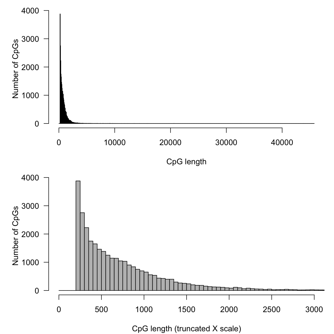
Distribution of lengths for all the CpG islands annotated in the Human genome.
Loading the Markov models
We start by loading the two Markov models previously computed from the RSAT tool create background model.
## Load a transition matrix from the RSAT result
readMarkovModel <- function(file) {
  model <- read.delim(
    file = file,
    row.names = 1)
  names(model) <- toupper(names(model))
  rownames(model) <- toupper(rownames(model))
  prior <- model[nrow(model),1:4] ## Last row contains priors as comments
  names(prior) <- names(model)[1:4]
  transitions <- rbind(model[1:4, 1:4], "B" = prior)
  return(transitions)
}

## Load the CpG transition table from the RSAT result
transitions.CpG <- readMarkovModel(file = "results/hg38/hg38_CpG_transitions_m1.tsv")

## Load the genomic background transition table from the RSAT result
transitions.Bg <- readMarkovModel(file = "results/hg38/hg38_genomic-bg_transitions_m1.tsv")

## Check that the rows of the transition matrix sum to 1
## (given some rounding errors)
# apply(transitions.CpG[2:5], 1, sum)
# apply(transitions.Bg[2:5], 1, sum)
## Define a function that draws a heatmap from a transition matrix
transition.heatmap <- function(
transitions,
main = "Transitions",
col.palette = gray.colors(n = 100, start = 1, end = 0),
breaks = (0:length(col.palette))/(n.colors*2)) {
n.colors <- length(col.palette)
h <- heatmap.2(
as.matrix(transitions),
main = main,
cellnote = round(digits = 3, as.matrix(transitions)),
trace = "none",
margins = c(4, 4),
# offsetRow = -10,
breaks = breaks,
key = FALSE,
srtCol = 0,
notecol = "black",
notecex = 1.2,
col = col.palette,
scale = "none",
las = 1,
Rowv = FALSE, Colv = FALSE, dendrogram = "none")
return(h)
# grab_grob()
}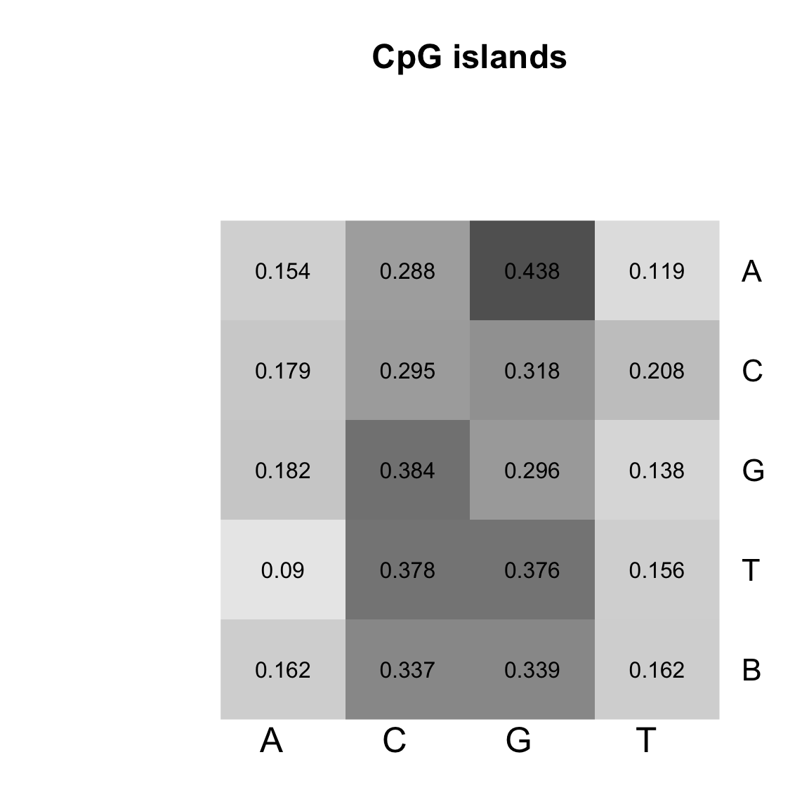
Heatmap of the transition matrices from 1st order Markov models trained on CpG islands.
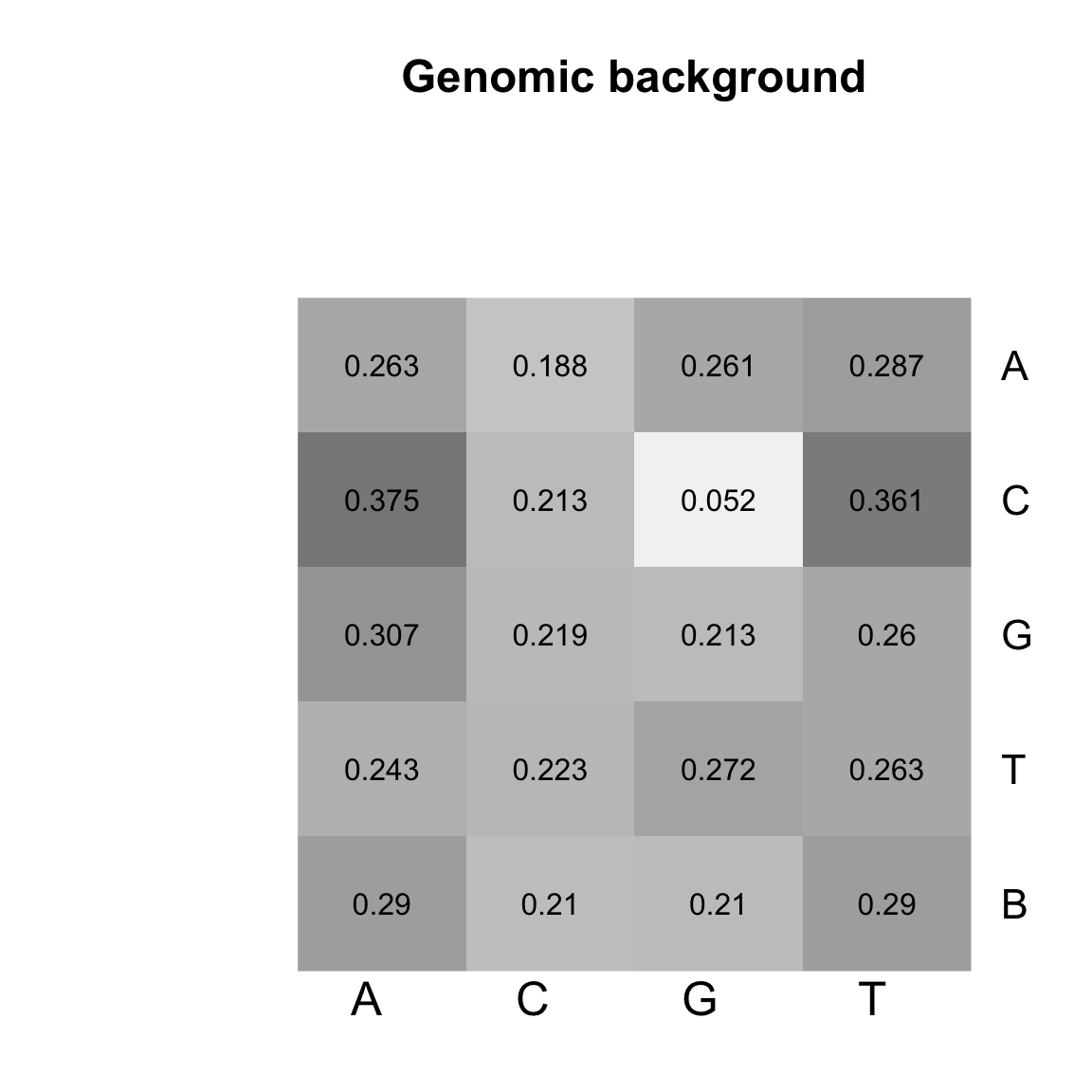
Heatmap of the transition matrices from 1st order Markov models trained on genomic background.
Discrimination between two models
Problem: for a given sequence of events (e.g. a nucleotidic sequence), identify the most likely Markov model.
Approach: compute the log-likelihood ratios (log-odd ratios) of the sequence probabilities computed using respectively the CpG island and genomic background models.
\[P_{\text{CpG}}(S) = P_{\text{CpG}}(S_1) \cdot \prod_{i=1}^{n-1} P_{\text{CpG}}(S_{i+1}|S_i)\] \[P_{\text{Bg}}(S) = P_{\text{Bg}}(S_1) \cdot \prod_{i=1}^{n-1} P_{\text{Bg}}(S_{i+1}|S_i)\]
\[L(S) = log \left( \frac{ P_{\text{CpG}}(S)}{P_{\text{Bg}}(S)} \right)\]
where
- \(L(S)\) is the log-likelihood of the sequence \(S\),
- \(P_{\text{CpG}}(S)\) the probability for this sequence to be generated by the CpG island model, and
- \(P_{\text{Bg}}(S)\) its probability to be generated by the background model.
A more efficient approach : rather than computing the two sequence probabilities (as the product of transition probabilities), we can compute once and forever a matrix with tbe log-odds of residue transitions.
\[L(r_j|r_i) = log \left( \frac{P_{\text{CpG}}(r_j|r_i)}{P_{\text{Bg}}(r_j|r_i)} \right)\]
my.palette <- colorRampPalette(c("blue", "white", "red"))(n = 100)

## Compute log-odds of transition frequencies
transition.log.odds <- log2(transitions.CpG / transitions.Bg)

max.lor <- ceiling(max(abs(range(transition.log.odds))))

heatmap.logodds <- transition.heatmap(
  transition.log.odds, "CpG / Bg log-odds",
  col.palette = my.palette,
#  breaks = seq(from = -max.lor, to = +max.lor, length.out = length(my.palette) + 1)
  breaks = length(my.palette) + 1
)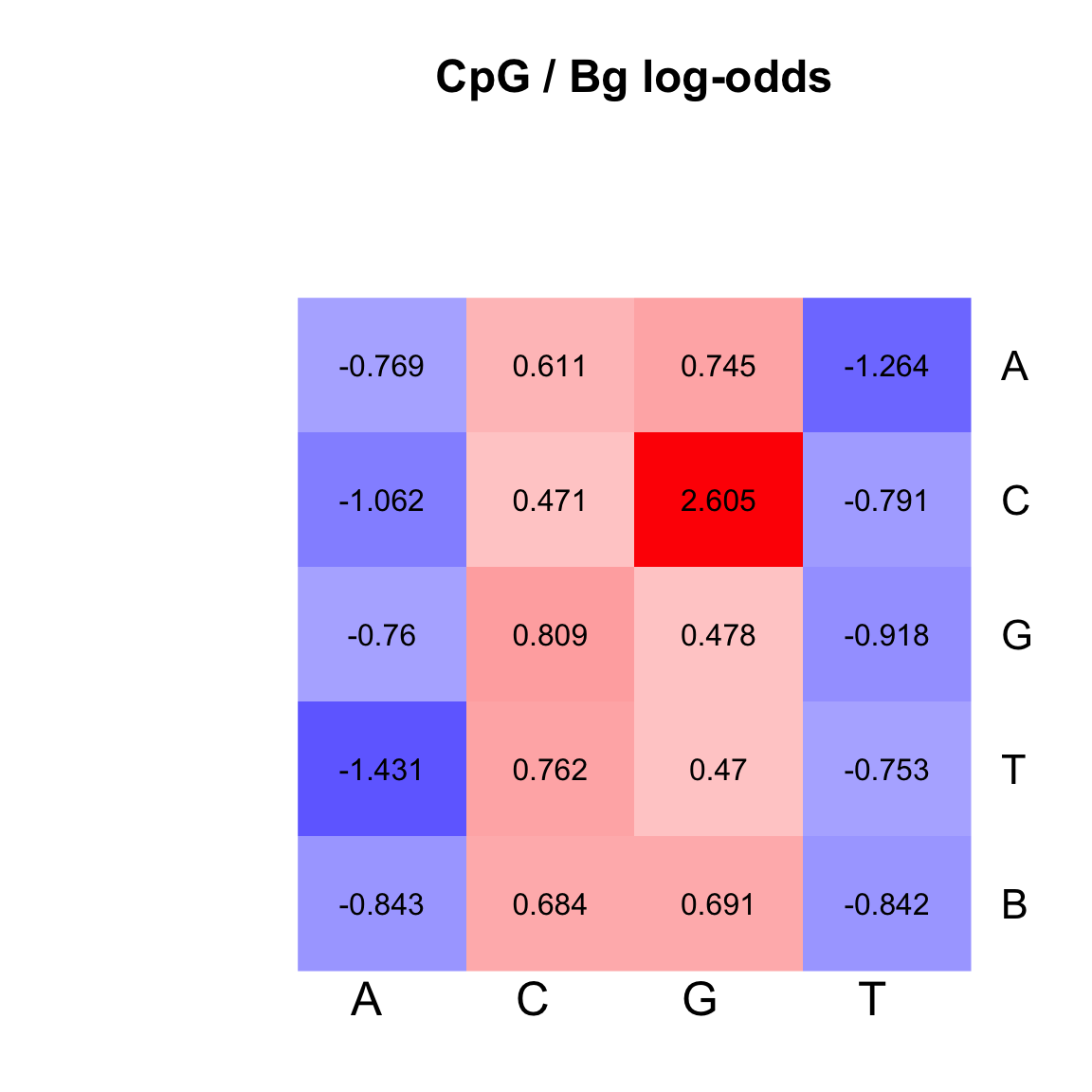
Heatmap of the log-odds between CpG and genomic background.
# library(gridGraphics)
# library(grid)
# library(gplots)
# library(gridExtra)
#
# grab_grob <- function(){
#   grid.echo()
#   grid.grab()
# }
# heatmaps <- list(
#   CpG = one.heatmap(transitions.CpG, "CpG islands"),
#   Bg = one.heatmap(transitions.Bg, "Genomic background")
# )
# grid.newpage()
# grid.arrange(grobs = heatmaps, ncol = 2, clip = TRUE)
We can then use this log-odds matrix to compute the log-odds of a sequence as the sum of the transition log-odds.
\[L(S) = L_{\text{B}}(S_1) \cdot \sum_{i=1}^{n-1} L(S_{i+1}|S_i)\]