Analysis of a genome annotation table
Probabilities and statistics for biology (STAT1)
Jacques van Helden
2019-10-26
Goal of this practical
During this practical session, you will run the following tasks:
- Handle a table containing annotated features of the yeast genome.
- Select a subset of the data by filtering rows based on a given criterion (annotation type, chromosome, …)
- Generate graphics to represent different aspects of the data.
- Compute estimators of central tendency and dispersion.
- Compute a confidence interval around the mean.
Expected report
At the end of the practical you will be asked to submit two documents
- Your R code.Each question must be explicitly formulated before presenting the results that answer it and giving an interpretation of these results.
- UA synthetic report, which will include a presentation of the main results (figures, descriptive stats, tables) as well as your interpretation of the result.
Expectation for the code
The code must be readable and undestandable: choose variable names that explicitly indicate what they represent.
The code must be properly documented (the
#symbol starts a comment, either at the beginning or in the middle of a line of code).Before each chunk of code, explain what this code is supposed to do, what it serves to.
Don’t hesitate to occasionally add some comment words to justify the chosen approach.
Each time you define a variable, add a comment on the same line to indicate what this variable represents.
The code must be portable: other people should be able to download it and run it on their computer. For this practical, I will systematically test whether your code can run on my computer. hard-coded absolute paths of a file on your machine should thus always be avoided (we will indicate hereafter how to define relative paths relative to the root of your user account).
Expected content for the interpretation report
Your report must be synthetic (1 text page max + as many figures and table as you wish)
Each question must be explicitly formulated before presenting the results that answer it and then interpreting those results.
Each figure or table must be documented with a legend that allows a naive reader to understand what it represents. The interpretation of the results displayed on a figure or table will be found in the main text (with a reference to the figure or table number).
Historical example: yeast genome
- 1992: publication of the first complete eukaryotic chromosome, the 3rd yeast chromosome.
- 1996: publication of the complete genome.
On the base of the genes of the 3rd chromosome (sample) we can estimate the average size of a yeast gene.
Questions:
Would the sample mean (chromosome III) be sufficient to predict the population mean (complete genome)?
To answer this question, we will imagine that we came back in 1992, and will use all the genes of chromosome III (considered here as a sample of the genome) to estimate the average size of genes for the whole genome (the “population” of genes").
Can this sample be described as “simple and independent”?
Analysis of the length of the baker’s yeast genes
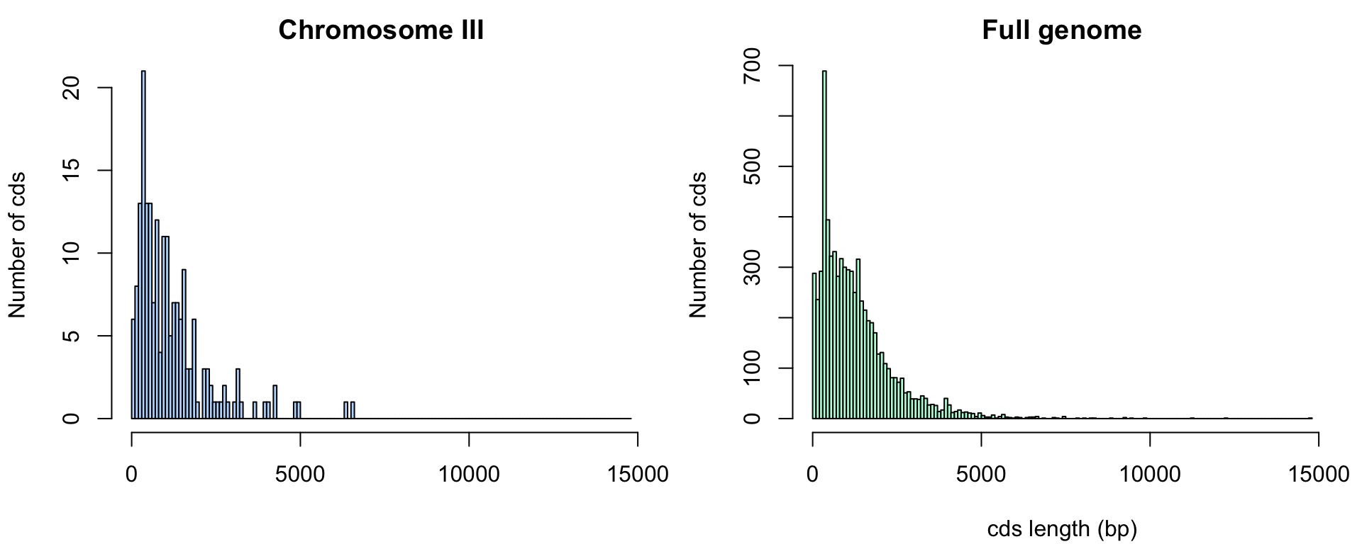
Distribution of cds lengths for Saccharomyces cerevisiae.
Tutorial
Before moving to the exercises, we show you here some basic elements about reading, manipulating and writing data tables with R.
The path to the home (manual)
We will create a folder for this tutorial, starting from the root of our account.
First possibility (quick but not very elegant): enter (manually) the path from the root of your account in a variable
dir.home <- /the/path/to/the/home
- Advantage: fast and convenient
- Disadvantage: not portable, will only work on your computer
The path to the home (automatic)
A more general solution: use the R command Sys.getenv().
- Invoked without parameters, this command lists all environment variables (your system configuration).
- The output can be restricted to a given environment variable, for example
Sys.getenv("HOME")returns the path to the root of your account.
Note: equivalent writing with Linux: the tilde symbol ~ also indicates the path to the root of your account.
## Identify the home directory
## by getting the environment variable HOME
dir.home <- Sys.getenv("HOME")
print(dir.home)
[1] "/Users/jvanheld"Creating a folder for the TP
## Define a variable containing the path of the results for this tutorial
dir.tuto <- file.path(dir.home, "stat1", "TP2")

print(dir.tuto)
[1] "/Users/jvanheld/stat1/TP2"## Create the directory for this tutorial
dir.create(path = dir.tuto,
showWarnings = FALSE,
recursive = TRUE)
## Go to the tutorial directory
setwd(dir.tuto)
## List the files already present in the folder (if any)
list.files()[1] "3nt_genomic_Saccharomyces_cerevisiae-ovlp-1str.tab"
[2] "chrom_sizes.tsv"
[3] "Saccharomyces_cerevisiae.R64-1-1.37.gtf.gz" Downloading the GTF file from EnsemblGenomes
Tips: before downloading the annotation file (GTF) from EnsemblGenomes to our computer, we will check if it is already present (and in this case we do not re-download it).
## Define the URL of the annotation file (GTF-formatted)
gtf.URL <- "ftp://ftp.ensemblgenomes.org/pub/release-37/fungi/gtf/saccharomyces_cerevisiae/Saccharomyces_cerevisiae.R64-1-1.37.gtf.gz"

## Define the path where the local copy will be stored
local.GTF <- file.path(dir.tuto, "Saccharomyces_cerevisiae.R64-1-1.37.gtf.gz")

## If the local file file laready exists, skip the download
if (file.exists(local.GTF)) {
  message("GTF file already exists in the tutorial folder: ", local.GTF)
} else {
  ## Download annotation table in GTF format
  download.file(url = gtf.URL, destfile = local.GTF)
  message("GTF file downloaded in the tutorial folder: ", local.GTF)
}
Loading a data table
R has several types of tabular structures (matrix, data.frame, table).
The most commonly used structure is the data.frame, which consists of an array of values (numeric or strings) whose rows and columns are associated with names.
The function read.table() allows you to read a text file containing a data table, and store the content in a variable.
Several functions derived from read.table() make it easier to read different types of formats:
read.delim()for files whose columns are delimited by a particular character (usually the tab, represented by ").read.csv()for files “comma-separated values”.
- Download the following file to your computer:
- Load it using the read.table function (for this you must replace the path below by that of your computer).
## Read a GTF file with yeast genome annotations

## Load the feature table
feature.table <- read.table(
  local.GTF,
  comment.char = "#",
  sep="\t",
  header=FALSE,
  row.names=NULL)

## The bed format does not contain any column header,
## so we set it manually based on the description of the format,
## found here:
##     http://www.ensembl.org/info/website/upload/gff.html
names(feature.table) <- c("seqname", "source", "feature", "start", "end", "score", "strand", "frame", "attribute")
Exploring the content of a data table
The first thing to do after loading a data table is to check its dimensions.
[1] 43028 9[1] 43028[1] 9The display of the complete annotation table would not be very readable, since it contains tens of thousands of lines.
We can display the first lines with the function head().
Note: the last column is particularly heavy (it contains a lot of information). We will see later how to select a subset of the columns to simplify the display.
  seqname source     feature start  end score strand frame
1      IV    SGD        gene  1802 2953     .      +     .
2      IV    SGD  transcript  1802 2953     .      +     .
3      IV    SGD        exon  1802 2953     .      +     .
4      IV    SGD         CDS  1802 2950     .      +     0
5      IV    SGD start_codon  1802 1804     .      +     0
                                                                                                                                                                                                                                    attribute
1                                                                                                                                                              gene_id YDL248W; gene_name COS7; gene_source SGD; gene_biotype protein_coding;
2                                                       gene_id YDL248W; transcript_id YDL248W; gene_name COS7; gene_source SGD; gene_biotype protein_coding; transcript_name COS7; transcript_source SGD; transcript_biotype protein_coding;
3                     gene_id YDL248W; transcript_id YDL248W; exon_number 1; gene_name COS7; gene_source SGD; gene_biotype protein_coding; transcript_name COS7; transcript_source SGD; transcript_biotype protein_coding; exon_id YDL248W.1;
4 gene_id YDL248W; transcript_id YDL248W; exon_number 1; gene_name COS7; gene_source SGD; gene_biotype protein_coding; transcript_name COS7; transcript_source SGD; transcript_biotype protein_coding; protein_id YDL248W; protein_version 1;
5                                        gene_id YDL248W; transcript_id YDL248W; exon_number 1; gene_name COS7; gene_source SGD; gene_biotype protein_coding; transcript_name COS7; transcript_source SGD; transcript_biotype protein_coding;
The function tail() displays the last few lines:
      seqname source     feature start   end score strand frame
43024    Mito    SGD  transcript 85554 85709     .      +     .
43025    Mito    SGD        exon 85554 85709     .      +     .
43026    Mito    SGD         CDS 85554 85706     .      +     0
43027    Mito    SGD start_codon 85554 85556     .      +     0
43028    Mito    SGD  stop_codon 85707 85709     .      +     0
                                                                                                                                                                                            attribute
43024                                                     gene_id Q0297; transcript_id Q0297; gene_source SGD; gene_biotype protein_coding; transcript_source SGD; transcript_biotype protein_coding;
43025                     gene_id Q0297; transcript_id Q0297; exon_number 1; gene_source SGD; gene_biotype protein_coding; transcript_source SGD; transcript_biotype protein_coding; exon_id Q0297.1;
43026 gene_id Q0297; transcript_id Q0297; exon_number 1; gene_source SGD; gene_biotype protein_coding; transcript_source SGD; transcript_biotype protein_coding; protein_id Q0297; protein_version 1;
43027                                      gene_id Q0297; transcript_id Q0297; exon_number 1; gene_source SGD; gene_biotype protein_coding; transcript_source SGD; transcript_biotype protein_coding;
43028                                      gene_id Q0297; transcript_id Q0297; exon_number 1; gene_source SGD; gene_biotype protein_coding; transcript_source SGD; transcript_biotype protein_coding;
If you are using the RStudio environment, you can display the table in a dynamic viewer pane with the function View().
Selection of subsets from a table
Selection of a line specified by its index.
   seqname source    feature start  end score strand frame
12      IV    SGD stop_codon  3834 3836     .      +     0
                                                                                                                                                            attribute
12 gene_id YDL247W-A; transcript_id YDL247W-A; exon_number 1; gene_source SGD; gene_biotype protein_coding; transcript_source SGD; transcript_biotype protein_coding;
Selection of a column specified by its index (display of the first values only).
[1] gene        transcript  exon        CDS         start_codon stop_codon
Levels: CDS exon gene start_codon stop_codon transcript
Selection of a cell by combining row and column indices.
[1] stop_codon
Levels: CDS exon gene start_codon stop_codon transcript
Selection of a column and/or row set.
    seqname source     feature start   end score
100      IV    SGD         CDS 34240 36477     .
101      IV    SGD start_codon 36475 36477     .
102      IV    SGD  stop_codon 34237 34239     .
103      IV    SGD        gene 36797 38173     .
104      IV    SGD  transcript 36797 38173     .
105      IV    SGD        exon 36797 38173     .
Selection of specific columns (here, the genomic coordinates of each feature): chromosome, beginning, end, strand.
    seqname start   end strand
100      IV 34240 36477      -
101      IV 36475 36477      -
102      IV 34237 34239      -
103      IV 36797 38173      +
104      IV 36797 38173      +
105      IV 36797 38173      +
Select a column based on its name.
  [1]  1802  1802  1802  1802  1802  2951  3762  3762  3762  3762  3762
 [12]  3834  5985  5985  5985  5985  5985  7812  8683  8683  8683  8686
 [23]  9754  8683 11657 11657 11657 11660 13358 11657 16204 16204 16204
 [34] 16204 16204 17224 17577 17577 17577 17580 18564 17577 18959 18959
 [45] 18959 18959 18959 19310 20635 20635 20635 20635 20635 21004 22471
 [56] 22471 22471 22474 22606 22471 22823 22823 22823 22823 22823 25874
 [67] 26403 26403 26403 26406 28773 26403 28985 28985 28985 28988 30452
 [78] 28985 30657 30657 30657 30657 30657 31827 32296 32296 32296 32296
 [89] 32296 33232 33415 33415 33415 33418 33916 33415 34237 34237 34237
[100] 34240
## Print the 20 first values of the "feature" field, which indicates the feature type
head(feature.table$feature, n = 20) [1] gene transcript exon CDS start_codon
[6] stop_codon gene transcript exon CDS
[11] start_codon stop_codon gene transcript exon
[16] CDS start_codon stop_codon gene transcript
Levels: CDS exon gene start_codon stop_codon transcriptSelection of several columns based on their names.
## Select the "start" column and print the 100 first results
feature.table[100:106, c("seqname", "start", "end", "strand")]
seqname start end strand
100 IV 34240 36477 -
101 IV 36475 36477 -
102 IV 34237 34239 -
103 IV 36797 38173 +
104 IV 36797 38173 +
105 IV 36797 38173 +
106 IV 36797 38170 +Note: Selection of several columns based on their names. It is also possible to name the rows of a data.frame but the GTF table does not support this. We will see more examples later.
Selection of a subset of rows based on the content of a column
The function subset() allows you to select a subset of the rows of a data.frame based on a condition applied to one or more columns.
We can apply it to select the subset of rows in the annotation table corresponding to coding sequences (CDS).
## Select subset of features having "cds" as "feature" attribute
cds <- subset(feature.table, feature == "CDS")

nrow(feature.table) ## Count the number of features
[1] 43028[1] 7050Count by value
The function table() allows you to count the occurrences of each value in a vector or array. Some examples of use below.
   I   II  III   IV   IX Mito    V   VI  VII VIII    X   XI  XII XIII  XIV
 759 2912 1210 5374 1567  327 2159  946 3856 2054 2617 2231 3789 3311 2774
  XV  XVI
3846 3296
        CDS        exon        gene start_codon  stop_codon  transcript
       7050        7872        7445        6700        6516        7445
We can use the knitr::kable() function to include a nicely formatted table in a report. This requires to load the knitr library.
## Count the number of features per type
require(knitr)
features.per.type <- table(feature.table$feature)

kable(features.per.type, col.names = c("feature type","Number"), caption = "Number of features of different types in the GTF annotations of the yest genome. ")| feature type | Number |
|---|---|
| CDS | 7050 |
| exon | 7872 |
| gene | 7445 |
| start_codon | 6700 |
| stop_codon | 6516 |
| transcript | 7445 |
Contingency tables can be calculated by counting the number of combinations between 2 vectors (or 2 columns of a table).
                I  II III  IV  IX Mito   V  VI VII VIII   X  XI XII XIII
  CDS         122 492 194 895 255   59 345 151 619  346 422 361 615  544
  exon        137 525 224 961 288   94 400 180 710  373 480 404 698  610
  gene        132 494 213 914 274   62 383 167 676  349 458 388 658  573
  start_codon 119 464 185 853 243   28 328 143 593  325 406 348 586  514
  stop_codon  117 443 181 837 233   22 320 138 582  312 393 342 574  497
  transcript  132 494 213 914 274   62 383 167 676  349 458 388 658  573

              XIV  XV XVI
  CDS         458 623 549
  exon        500 689 599
  gene        475 665 564
  start_codon 438 607 520
  stop_codon  428 597 500
transcript 475 665 564 feature
seqname CDS exon gene start_codon stop_codon transcript
I 122 137 132 119 117 132
II 492 525 494 464 443 494
III 194 224 213 185 181 213
IV 895 961 914 853 837 914
IX 255 288 274 243 233 274
Mito 59 94 62 28 22 62
V 345 400 383 328 320 383
VI 151 180 167 143 138 167
VII 619 710 676 593 582 676
VIII 346 373 349 325 312 349
X 422 480 458 406 393 458
XI 361 404 388 348 342 388
XII 615 698 658 586 574 658
XIII 544 610 573 514 497 573
XIV 458 500 475 438 428 475
XV 623 689 665 607 597 665
XVI 549 599 564 520 500 564| CDS | exon | gene | start_codon | stop_codon | transcript | |
|---|---|---|---|---|---|---|
| I | 122 | 137 | 132 | 119 | 117 | 132 |
| II | 492 | 525 | 494 | 464 | 443 | 494 |
| III | 194 | 224 | 213 | 185 | 181 | 213 |
| IV | 895 | 961 | 914 | 853 | 837 | 914 |
| IX | 255 | 288 | 274 | 243 | 233 | 274 |
| Mito | 59 | 94 | 62 | 28 | 22 | 62 |
| V | 345 | 400 | 383 | 328 | 320 | 383 |
| VI | 151 | 180 | 167 | 143 | 138 | 167 |
| VII | 619 | 710 | 676 | 593 | 582 | 676 |
| VIII | 346 | 373 | 349 | 325 | 312 | 349 |
| X | 422 | 480 | 458 | 406 | 393 | 458 |
| XI | 361 | 404 | 388 | 348 | 342 | 388 |
| XII | 615 | 698 | 658 | 586 | 574 | 658 |
| XIII | 544 | 610 | 573 | 514 | 497 | 573 |
| XIV | 458 | 500 | 475 | 438 | 428 | 475 |
| XV | 623 | 689 | 665 | 607 | 597 | 665 |
| XVI | 549 | 599 | 564 | 520 | 500 | 564 |
Exercises
1. GTF format specifications
Read the GTF format specifications.
2. Creating a local folder for the TP
Create a local folder (for example: stat1/TP_yeast from the root of your account). We suggest you to use the following functions.
Sys.getenv("HOME")(Linux and Mac OS X), to get the root of your user account;file.path()to build a path;dir.create()to create the folder for the TP. Read carefully the options of this function withhelp(dir.create)
(solution is above)
3. Locating the annotation file
Locate the yeast genome annotation file in GTF format in this local folder.
- Site Ensembl Fungi: http://fungi.ensembl.org/
- Click “Downloads” to access the ftp website
- In the search box, type “saccharomyces cerevisiae” and follow the link “GTF”
- Copy the address (URL) of the file Saccharomyces_cerevisiae.R64-1-1.37.gtf.gz
(solution above)
4. Downloading a file from an ftp website
Suggested functions:
download.file()(read the help to know the arguments)
(solution above)
5. Loading a data table in R
Write a script that loads the data table into a variable named feature.table, using the function R read.delim().
Be sure to ignore the comment lines (which start with a character #).
(solution above)
6. Compute the length of coding genes
- Add to the annotation table (
feature.table) a column entitled “length” which indicates the length of each annotated genomic feature.
## Add a colmn with feature lengths
feature.table[, "length"] <- feature.table[, "end"] - feature.table[, "start"] + 1

## Add a colmn with feature lengths: equivalent result with simpler notation
feature.table$length <- feature.table$end - feature.table$start + 1
Count the number of rows in the table corresponding to each type of annotation (3rd column of the GTF, “feature”).
- fonction
table()
- fonction
        CDS        exon        gene start_codon  stop_codon  transcript
7050 7872 7445 6700 6516 7445 - Print the same result in a nicely formatted table with
knitr::kable()./
| Var1 | Freq |
|---|---|
| CDS | 7050 |
| exon | 7872 |
| gene | 7445 |
| start_codon | 6700 |
| stop_codon | 6516 |
| transcript | 7445 |
Select the lines corresponding to coding regions (“CDS”)
- fonction
subset()
- fonction
Count the number of CDS per chromosome.
- fonction
table()
- fonction
   I   II  III   IV   IX Mito    V   VI  VII VIII    X   XI  XII XIII  XIV
 122  492  194  895  255   59  345  151  619  346  422  361  615  544  458
  XV  XVI
623 549 | Chromosome | Number of CDSs |
|---|---|
| I | 122 |
| II | 492 |
| III | 194 |
| IV | 895 |
| IX | 255 |
| Mito | 59 |
| V | 345 |
| VI | 151 |
| VII | 619 |
| VIII | 346 |
| X | 422 |
| XI | 361 |
| XII | 615 |
| XIII | 544 |
| XIV | 458 |
| XV | 623 |
| XVI | 549 |
- Load the chromosome size table chrom_sizes.tsv, and compute the density of genes for each chromosome (number of genes per Mb).
[1] 316617[1] 7445[1] 7050
6. Histogram of gene length
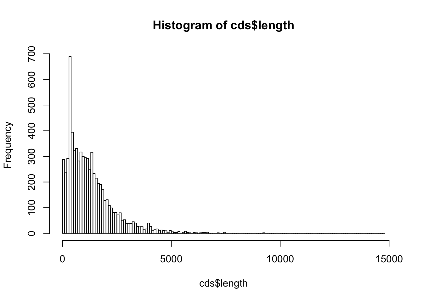
By using the function hist(), draw a histogram representing the length distribution of the CDS.

Choose the class intervals in a way that the histogram is informative (neither too large nor too few classes).
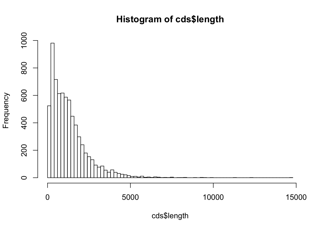
Retrieve the result of hist() in a variable named cds.length.hist.
Print the result on the screen (print()) and analyze the structure of the variable cds.length.hist (this is a list variable).
Useful functions:
$breaks
  [1]     0   100   200   300   400   500   600   700   800   900  1000
 [12]  1100  1200  1300  1400  1500  1600  1700  1800  1900  2000  2100
 [23]  2200  2300  2400  2500  2600  2700  2800  2900  3000  3100  3200
 [34]  3300  3400  3500  3600  3700  3800  3900  4000  4100  4200  4300
 [45]  4400  4500  4600  4700  4800  4900  5000  5100  5200  5300  5400
 [56]  5500  5600  5700  5800  5900  6000  6100  6200  6300  6400  6500
 [67]  6600  6700  6800  6900  7000  7100  7200  7300  7400  7500  7600
 [78]  7700  7800  7900  8000  8100  8200  8300  8400  8500  8600  8700
 [89]  8800  8900  9000  9100  9200  9300  9400  9500  9600  9700  9800
[100]  9900 10000 10100 10200 10300 10400 10500 10600 10700 10800 10900
[111] 11000 11100 11200 11300 11400 11500 11600 11700 11800 11900 12000
[122] 12100 12200 12300 12400 12500 12600 12700 12800 12900 13000 13100
[133] 13200 13300 13400 13500 13600 13700 13800 13900 14000 14100 14200
[144] 14300 14400 14500 14600 14700 14800

$counts
  [1] 288 236 292 689 394 322 331 282 317 300 295 292 250 316 233 215 194
 [18] 190 170 128 131 109  99  81  81  72  80  51  53  39  39  38  45  40
 [35]  27  28  26  14  17  40  27  12  14  17  12  13  11  10   4  11   6
 [52]   3   3   7   1   4   8   3   2   1   3   2   0   2   3   3   4   0
 [69]   1   0   0   2   1   0   4   0   0   0   1   0   1   0   1   1   0
 [86]   0   0   0   1   0   0   0   2   0   1   0   0   0   1   0   0   0
[103]   0   0   0   0   0   0   0   0   0   0   1   0   0   0   0   0   0
[120]   0   0   0   1   0   0   0   0   0   0   0   0   0   0   0   0   0
[137]   0   0   0   0   0   0   0   0   0   0   0   1

$density
  [1] 4.085106e-04 3.347518e-04 4.141844e-04 9.773050e-04 5.588652e-04
  [6] 4.567376e-04 4.695035e-04 4.000000e-04 4.496454e-04 4.255319e-04
 [11] 4.184397e-04 4.141844e-04 3.546099e-04 4.482270e-04 3.304965e-04
 [16] 3.049645e-04 2.751773e-04 2.695035e-04 2.411348e-04 1.815603e-04
 [21] 1.858156e-04 1.546099e-04 1.404255e-04 1.148936e-04 1.148936e-04
 [26] 1.021277e-04 1.134752e-04 7.234043e-05 7.517730e-05 5.531915e-05
 [31] 5.531915e-05 5.390071e-05 6.382979e-05 5.673759e-05 3.829787e-05
 [36] 3.971631e-05 3.687943e-05 1.985816e-05 2.411348e-05 5.673759e-05
 [41] 3.829787e-05 1.702128e-05 1.985816e-05 2.411348e-05 1.702128e-05
 [46] 1.843972e-05 1.560284e-05 1.418440e-05 5.673759e-06 1.560284e-05
 [51] 8.510638e-06 4.255319e-06 4.255319e-06 9.929078e-06 1.418440e-06
 [56] 5.673759e-06 1.134752e-05 4.255319e-06 2.836879e-06 1.418440e-06
 [61] 4.255319e-06 2.836879e-06 0.000000e+00 2.836879e-06 4.255319e-06
 [66] 4.255319e-06 5.673759e-06 0.000000e+00 1.418440e-06 0.000000e+00
 [71] 0.000000e+00 2.836879e-06 1.418440e-06 0.000000e+00 5.673759e-06
 [76] 0.000000e+00 0.000000e+00 0.000000e+00 1.418440e-06 0.000000e+00
 [81] 1.418440e-06 0.000000e+00 1.418440e-06 1.418440e-06 0.000000e+00
 [86] 0.000000e+00 0.000000e+00 0.000000e+00 1.418440e-06 0.000000e+00
 [91] 0.000000e+00 0.000000e+00 2.836879e-06 0.000000e+00 1.418440e-06
 [96] 0.000000e+00 0.000000e+00 0.000000e+00 1.418440e-06 0.000000e+00
[101] 0.000000e+00 0.000000e+00 0.000000e+00 0.000000e+00 0.000000e+00
[106] 0.000000e+00 0.000000e+00 0.000000e+00 0.000000e+00 0.000000e+00
[111] 0.000000e+00 0.000000e+00 1.418440e-06 0.000000e+00 0.000000e+00
[116] 0.000000e+00 0.000000e+00 0.000000e+00 0.000000e+00 0.000000e+00
[121] 0.000000e+00 0.000000e+00 1.418440e-06 0.000000e+00 0.000000e+00
[126] 0.000000e+00 0.000000e+00 0.000000e+00 0.000000e+00 0.000000e+00
[131] 0.000000e+00 0.000000e+00 0.000000e+00 0.000000e+00 0.000000e+00
[136] 0.000000e+00 0.000000e+00 0.000000e+00 0.000000e+00 0.000000e+00
[141] 0.000000e+00 0.000000e+00 0.000000e+00 0.000000e+00 0.000000e+00
[146] 0.000000e+00 0.000000e+00 1.418440e-06

$mids
  [1]    50   150   250   350   450   550   650   750   850   950  1050
 [12]  1150  1250  1350  1450  1550  1650  1750  1850  1950  2050  2150
 [23]  2250  2350  2450  2550  2650  2750  2850  2950  3050  3150  3250
 [34]  3350  3450  3550  3650  3750  3850  3950  4050  4150  4250  4350
 [45]  4450  4550  4650  4750  4850  4950  5050  5150  5250  5350  5450
 [56]  5550  5650  5750  5850  5950  6050  6150  6250  6350  6450  6550
 [67]  6650  6750  6850  6950  7050  7150  7250  7350  7450  7550  7650
 [78]  7750  7850  7950  8050  8150  8250  8350  8450  8550  8650  8750
 [89]  8850  8950  9050  9150  9250  9350  9450  9550  9650  9750  9850
[100]  9950 10050 10150 10250 10350 10450 10550 10650 10750 10850 10950
[111] 11050 11150 11250 11350 11450 11550 11650 11750 11850 11950 12050
[122] 12150 12250 12350 12450 12550 12650 12750 12850 12950 13050 13150
[133] 13250 13350 13450 13550 13650 13750 13850 13950 14050 14150 14250
[144] 14350 14450 14550 14650 14750

$xname
[1] "cds$length"

$equidist
[1] TRUE

attr(,"class")
[1] "histogram"class(cds.length.hist)attributes(cds.length.hist)
Other types of graphs allow you to explore the distribution of a set of data. In particular, box plots display, for a series of data, the median, the quarterfinal range, a confidence interval and outliers.
In the boxplot() function, we use the formula length ~ seqname in order to group lengths by seqname (i.e. chromosome names).
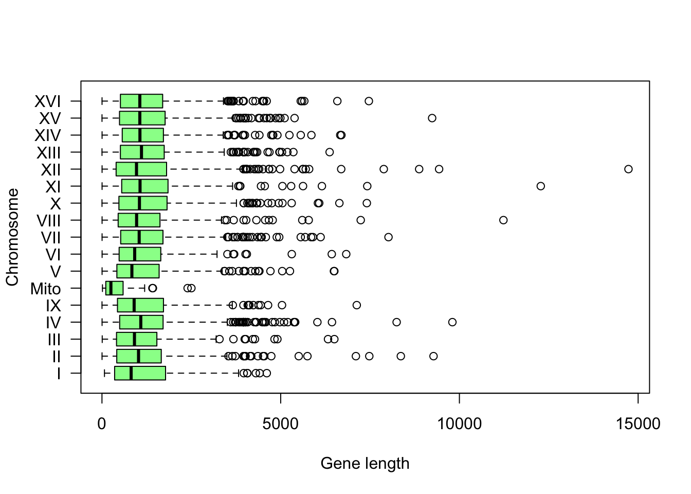
Boîte à moustache indiquant la distribution de longueur des gènes par chromosome.
7. Descriptive parameters
Calculate the parameters of central tendency (mean, median, mode) and dispersion (variance, standard deviation, inter-quarterly deviation)
- for the genes of chromosome III;
- for all yeast genes.
[1] 194 1[1] "data.frame"[1] "numeric"length1 length2 length3 length4 length5 length6
741 1845 1374 780 630 525 [1] "Chromosome III contains 194 CDS"[1] 1169.521Ah ah! (skeptical tone) The R function sd() does not compute the standard deviation of the input numbers (\(s\)), but the estimate of the standard deviaiton of the population (\(\hat{\sigma}\))
Display these parameters on the histogram of gene length, using the function arrows()
8. Confidence interval
From genes of chromosome III (considered as the sample available in 1992), calculate a confidence interval around the mean, and formulate the interpretation of this confidence interval. Then evaluate whether or not this confidence interval covered the average population (all genes in the yeast genome, which became available 4 years after chromosome III).
\[ \bar{x} \pm \frac{\hat{\sigma}}{\sqrt(n)} \cdot t_{1-\alpha/2}^{n-1}\]
[1] -1.972332Draw a polygon of frequencies indicating the number of genes per class (class medium).
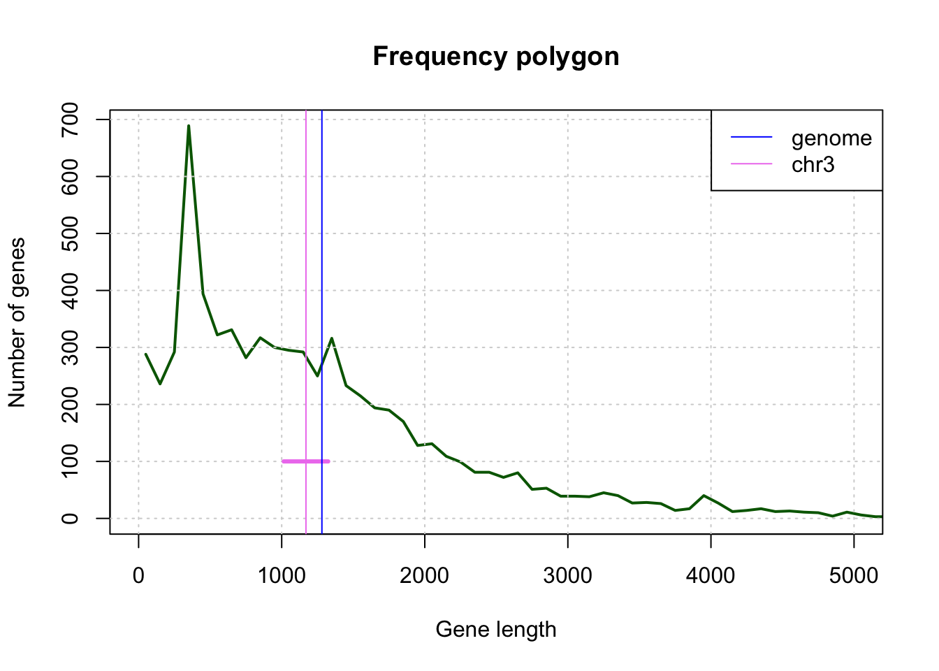
9. Distribution of gene length
From the result of
hist(), retrieve an array (in a variable of typedata.frame) indicating the absolute frequencies (count) according to the median class size (mids),Add to this table a column indicating the relative frequency of each class of gene length.
Add columns to this table indicating the empirical distribution function gene lengths (number of genes of a size less than or equal to each observed \(x\) value, and relative frequency of this number).
- basic function:
cumsum() - advanced function:
ecdf()
- basic function:
by using the functions
plot()andlines(), draw a graph representing the absolute frequency per class (medians of classes in \(X\), counts in \(Y\)), and the empirical distribution function.- suggestion: superposez les ??utilisez le type de lignes “h” pour les fréquences de classe, et “l” ou “s” pour la fonction de répartition.
10. Expected distribution of gene lengths
Based on the genome size (\(12.156.679\) bp) and genomic frequencies of the codons provided in the table below, calculate the gene length distribution that would be expected by chance, and draw it on top of the graph with the observed distribution of gene lengths.
Note: the genomic frequencies of all polynucleotides can be downloaded here: 3nt_genomic_Saccharomyces_cerevisiae-ovlp-1str.tab
Alternative: create a variable freq.3nt and manually assign the values for the 4? required polynucleotides from the table below.
| sequence | frequency | occurrences |
|---|---|---|
| AAA | 0.0394 | 478708 |
| ATG | 0.0183 | 221902 |
| TAA | 0.0224 | 272041 |
| TAG | 0.0129 | 156668 |
| TGA | 0.0201 | 244627 |
| TTT | 0.0391 | 475658 |
## Compute the probabilities of start, stop ,and not-stop codons
P <- c("start" = oligo.freq["ATG", "frequency"],
       "stop" = sum(oligo.freq[c("TAA", "TGA", "TAG"), "frequency"])
       )
P["not-stop"] <- 1 - P["stop"]


## Rounded number encompassing the number of codons of the longest gene
max.n <- 100 * ceiling(max(cds$length) / 300)
n <- 1:max.n # A vector with all relevant length in numbers of codons
L <- 3*n # Gene lengths in base pairs

## Probability of observing an ORF of exactly n codons
length.proba.density <- P["start"] * P["not-stop"]^n * P["stop"]
length.pvalue <- rev(cumsum(rev(length.proba.density)))

## Compute the random expectation for the number of genes
## Note: genes can be found on both strands -> we multiply by 2
G <- 12156679 ## Genome length
exp.genes <- length.pvalue * G * 2


## Plot the open reading frame (ORF) probability as a
## function of ORF length (in base pairs)
par(mfrow = c(3,2))
plot(L, length.proba.density, type = "h",
     las = 1, col = "blue",
     main = "ORF length probability density (full range)",
     xlab = "ORF length (base pairs)",
     ylab = "P(X = x)")

plot(L, length.proba.density, type = "h", xlim = c(0,600),
     las = 1, col = "blue",
     main = "ORF length probability density (restricted range)",
     xlab = "ORF length (base pairs)",
     ylab = "P(X = x)")

plot(L, length.pvalue, type = "l", xlim = c(0,600),
     las = 1, col = "darkgreen", lwd = 2, panel.first = grid(),
     main = "ORF length P-value",
     xlab = "ORF length (base pairs)",
     ylab = "P(X >= x)")

plot(L, exp.genes, type = "l", xlim = c(0,600),
     las = 1, col = "darkgreen", lwd = 2, panel.first = grid(),
     main = "Expected number of ORFs (restricted range)",
     xlab = "ORF length (base pairs)",
     ylab = "Expected ORFs")

plot(L, length.pvalue, type = "l",
     las = 1, col = "darkgreen", lwd = 2, panel.first = grid(),
     log = "y", xlim = c(0, 600), ylim = c(length.pvalue[201], 1),
     main = "ORF length P-value",
     xlab = "ORF length (base pairs)",
     ylab = "P(X >= x) on a log scale")

plot(L, exp.genes, type = "l",
     las = 1, col = "darkgreen", lwd = 2, panel.first = grid(),
     log = "y", xlim = c(0, 600), ylim = c(exp.genes[201], exp.genes[1]),
     main = "ORF length E-value (restricted range)",
     xlab = "ORF length (base pairs)",
     ylab = "Expected ORFs (log scale)")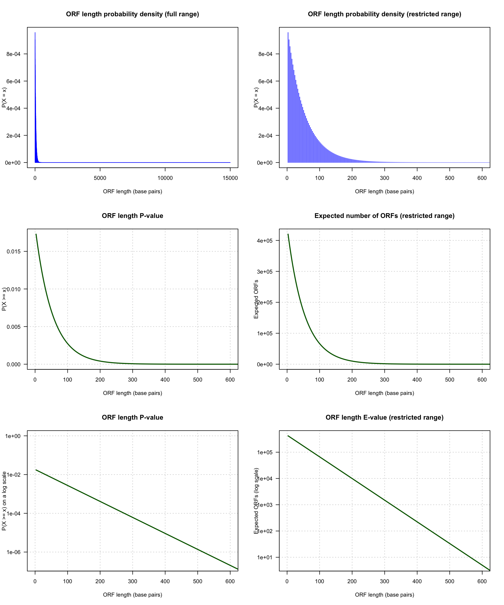
Distribution of the number of ORFs expected by chance in a random genomic sequence having the same codon frequencies as the yeast genome.
The top-left panel shows the density of probability of ORF lengths, i.e. the probability to observe by chance an ORF of exactly \(x\) nucleotides: \(P(X = x)\). The shape of the distribution is not very well depicted because the range extends up to \(15,000\) base pairs, the length of the longest yeast gene. This gene is an outlier (exceptionally long, not representative of the other yeast genes).
The top right panel shows the same distribution with a range restricted to 0-600 bp.
The middle left panel shows the distribution of P-value for ORF lengths \(x\) ranging from 0 to 600: \(P(X \ge x)\). This is the probability, for each length \(x\), to find by chance a gene at least as long starting at a given genomic position.
The middle right panel shows the E-value \(E(X \ge x)\), i.e. the number of ORFs expected by chance in the whole genome, for length \(x\) ranging from 0 to 600.
The bottom panels show the same distributions of P-value (left) and E-value (right) on a logarithmic scale, to better emphasize the very small probabilities.
Of note, with a threshold \(X \ge 300\), we still expect 1489.6702982 ORFs at random. Since this threshold was used to infer the presence of an ORF in the original annotation of the yeast genome, biologists knew that these annotations would contain an important number of false ORF predictions. Consistently, several hundreds of genes were discarded from the annotations a few years later, based on comparative genomics. Indeed, when the genomes of other fungal species became available, the genes for which no homologs was found in any other fungal genome were considered likely false positives.
11. Before finishing: keep track of your session
Tractability is an essential issue in science. The function R sessionInfo() provides a summary of the conditions of a work session: version of R, operator system, libraries of functions used.
R version 3.6.1 (2019-07-05)
Platform: x86_64-apple-darwin15.6.0 (64-bit)
Running under: macOS Mojave 10.14.6

Matrix products: default
BLAS:   /Library/Frameworks/R.framework/Versions/3.6/Resources/lib/libRblas.0.dylib
LAPACK: /Library/Frameworks/R.framework/Versions/3.6/Resources/lib/libRlapack.dylib

locale:
[1] en_US.UTF-8/en_US.UTF-8/en_US.UTF-8/C/en_US.UTF-8/en_US.UTF-8

attached base packages:
[1] stats     graphics  grDevices utils     datasets  methods   base

other attached packages:
[1] knitr_1.25

loaded via a namespace (and not attached):
 [1] compiler_3.6.1  magrittr_1.5    tools_3.6.1     htmltools_0.4.0
 [5] yaml_2.2.0      Rcpp_1.0.2      stringi_1.4.3   rmarkdown_1.16
 [9] highr_0.8       stringr_1.4.0   xfun_0.10       digest_0.6.21
[13] rlang_0.4.0     evaluate_0.14