Practical – Microarray analysis – Data loading and exploration
(STAT2)
Jacques van Helden
2020-04-12
####  Define Local directories and files for the data and result ####

## Find the home directory
myHome <- Sys.getenv("HOME")

## Define the main directory for the  data and results
mainDir <- file.path(myHome,
                     "STAT2_CMB_practicals",
                     "den-boer-2009")
dir.create(path = mainDir)
message("Main dir: ", mainDir)

## Define a file where we wills tore the memory image
memImageFile <- file.path(mainDir, "DenBoerData_loaded.Rdata")

## Define the dir where we will download the data
dataDir <- file.path(mainDir, "data")
message("Local data dir: ", dataDir)
Introduction
In this practical, we will load a dataset that will be used as study case to apply different approaches of multivariate analysis:
- data exploration
- multidimensional scaling
- differential analysis
- clustering (unsupervised classification)
- supervised classification
Study case
Reference: Den Boer ML et al. (2009). A subtype of childhood acute lymphoblastic leukaemia with poor treatment outcome: a genome-wide classification study. Lancet Oncol. 2009 10:125-34.
- DOI: [doi: 10.1016/S1470-2045(08)70339-5]
- Pubmed: [PMID 19138562].
- Raw data available at Gene Expression Omnibus, series [GSE13425]
- Preprocessed data: https://github.com/jvanheld/stat1/raw/master/data/DenBoer_2009/.
Data pre-processing
The raw microarray data has been pre-processed in order to dispose of a ready-to-use dataset. pre-processing included
- filtering of barely detected or poorly expressed genes,
- log2 transformation to normalise the raw measurements
- between-sample standardisation to enable comparison between the different samples.
Availability of the pre-processed data
The preprocessed data is available here: https://github.com/jvanheld/stat1/raw/master/data/DenBoer_2009/.
It contains the following files.
| File | Contents | Structure |
|---|---|---|
| GSE13425_group_descriptions.tsv.gz | Description of the patient groups | Tab-delimited file with one row per group and one column per type of description (group name, label) |
| phenoData_GSE13425.tsv.gz | Metadata (sample descriptions) | Tab-delimited file with one row per biological sample (one per patient) and one column per type of information about the biological sample |
| GSE13425_Norm_Whole.tsv.gz | Normalised microarray data | Tab-delimited file with one row per gene and one column per patient |
| GSE13425_AMP_Whole.tsv.gz | Detection status of each gene in each sample (Absent, Marginal, Present) | Tab-delimited file with one row per gene and one column per patient |
Data download
Write an R script that perform the following operations
- Creates a directory to store a local copy for this practical on your computer. (
~/STAT2_CMB_practicals/den-boer-2009/). - Creates a sub-directory for the data (
~/STAT2_CMB_practicals/den-boer-2009/data/). - Lists the files available on the data Web site (https://github.com/jvanheld/stat1/raw/master/data/DenBoer_2009/).
- For each of these files, checkS if it is already present in your local local data directory, and downloads it if it is not the case.
Try to make your code re-usable, in the perspective to apply it soon in order to download data sets from other web sites.
#' @title Download a set of files from a Web site
#' @author Jacques van Helden
#' @description Download a set of files from a Web site and store them in a destination directory if they do not exist yet there.
#' @param files a vector with the file names
#' @param dataURL the URL of the folder containing the files to download
#' @param destDir local destination directory. Will be created if it does not exist.
#' @return no return value
#' @export
DownloadMyFiles <- function(files,
                            dataURL,
                            destDir) {

  ## Create local directory
  dir.create(destDir, recursive = TRUE, showWarnings = FALSE)

  for (f in files) {

    ## Destination file
    destFile <- file.path(destDir, f)

    ## Check if file exists
    if (file.exists(destFile)) {
      message("skipping download because file exists: ", destFile)
    } else {
      sourceURL <- file.path(dataURL, f)
      download.file(url = sourceURL, destfile = destFile)
    }
  }
}
## URL of the folder containing the data fle
dataURL <- "https://github.com/jvanheld/stat1/raw/master/data/DenBoer_2009/"
files <- c(
expr = "GSE13425_Norm_Whole.tsv.gz",
pheno = "phenoData_GSE13425.tsv.gz",
groups = "GSE13425_group_descriptions.tsv.gz"
)
# ## Local data dir
# destDir <- "~/STAT2_CMB_practicals/den-boer-2009/data/"
## Call the function to download the files
DownloadMyFiles(files = files, dataURL = dataURL, destDir = dataDir)
kable(data.frame(list.files(dataDir)),
caption = "Content of the destination directory after file download. ")| list.files.dataDir. |
|---|
| GSE13425_group_descriptions.tsv.gz |
| GSE13425_Norm_Whole.tsv.gz |
| phenoData_GSE13425.tsv.gz |
Data loading
Write an R script that loads the data tables from your local data directory.
Some indication about the checks we do when we load the data tables.
Load the expression table in a data frame named
exprTable, with one row per gene, one column per sample. Tip: row names should indicate gene names, and column names the sample IDs.Load the metadata in a table named
phenoTable, with one row per sample and one column per description field. Tip: row name should indicate sample names.Check that the samples have the same order in the columns of the expression table and the rows of the pheno table.
Create a vector named
sampleGroupwith the group membership of each sample. Tip: don’t forget to convert the factor (coming from the data.frame column) into a vector.Load the group descriptions in a data frame named
groupDescriptions, with one row per group.
#### Load data tables ####
message("Loading data tables")

## Load expression table
message("\tLoading expression table")
exprTable <- read.table(file.path(dataDir, files["expr"]),
                        sep = "\t",
                        header = TRUE,
                        quote = "",
                        row.names = 1)
# dim(exprTable)
# names(exprTable)
# head(exprTable)

## Compute the number of samples (columns) and genes (rows) in the expression table
nbSamples <- ncol(exprTable)
nbGenes <- nrow(exprTable)

## Load metadescriptions (pheno table)
message("\tLoading metadata table (pheno)")
phenoTable <- read.table(file.path(dataDir, files["pheno"]),
                         sep = "\t",
                         header = TRUE,
                         quote = "",
                         row.names = 1)
# dim(phenoTable)
# View(phenoTable)
# names(phenoTable)
sampleGroup <- as.vector(phenoTable$Sample.title)

## Load group descriptions
message("\tLoading group descriptions")
groupDescriptions <- read.table(file.path(dataDir, files["groups"]),
                                sep = "\t",
                                header = TRUE,
                                quote = "",
                                row.names = 1)
# dim(phenoTable)

## Define a color and label for each sample
sampleColor <-  as.vector(phenoTable$sample.colors)
sampleLabel <-  as.vector(phenoTable$sample.labels)


#### Number of samples per group ####

## Count the number of biological samples per cancer group
samplesPerGroup <- table(sampleGroup)

## Add a column with group sizes
groupDescriptions[, "samples"] <- samplesPerGroup[rownames(groupDescriptions)]

## Sort the group description table by decreasing size
groupDescriptions <- groupDescriptions[order(groupDescriptions$samples, decreasing = TRUE), ]

#### Print a table with group descriptions  ####
kable(groupDescriptions)| group.labels | group.colors | samples | |
|---|---|---|---|
| hyperdiploid | Bh | brown | 44 |
| pre-B ALL | Bo | darkblue | 44 |
| TEL-AML1 | Bt | red | 43 |
| T-ALL | T | darkgreen | 36 |
| E2A-rearranged (EP) | BEp | orange | 8 |
| E2A-rearranged (E-sub) | BEs | darkgray | 4 |
| BCR-ABL | Bc | cyan | 4 |
| MLL | BM | violet | 4 |
| TEL-AML1 + hyperdiploidy | Bth | blue | 1 |
| E2A-rearranged (E) | BE | green | 1 |
| BCR-ABL + hyperdiploidy | Bch | black | 1 |
The expression table has been loaded in a data.frame named exprTable, which contains
- 22283 variables (rows) representing gens
- 190 individuals (columns) corresponding to biological samples.
The metadata (“pheno” table) contains 190 rows and 6 columns.
Marginal statistics
Write an R script that computes marginal statistics (mean, standard deviation, variance, min, percentiles 5, 10, 25, 50, 75, 90, 95, max, IQR) on each row of the normalised data table (one row corresponds to one gene).
Do the same for each column (patient).
Tips:
- Use the function
apply()to compute statistics on each row (margin = 1) or column (margin = 2) of a data.frame. - Since the function
apply()returns a vector, one possibility would be to store in separate vectors the mean, sd, var, min, etc. However it will be more convenient to regroup all the statistics in a single data frame with one row per object of interest (individuals or variables, depending on whether we compute margins on columns or rows, resp.) and one column per statistics (mean, sd, var, mean, …). This can be done with thedata.frame()function.
#### Compute statistics on each column ####
message("Computing column statistics")
colStat <- data.frame(
  mean = apply(exprTable, 2, mean, na.rm = TRUE),
  var = apply(exprTable, 2, var, na.rm = TRUE),
  sd = apply(exprTable, 2, sd, na.rm = TRUE),
  min = apply(exprTable, 2, min, na.rm = TRUE),
  perc05 = apply(exprTable, 2, quantile, probs = 0.05, na.rm = TRUE),
  perc25 = apply(exprTable, 2, quantile, probs = 0.25, na.rm = TRUE),
  perc50 = apply(exprTable, 2, quantile, probs = 0.50, na.rm = TRUE),
  perc75 = apply(exprTable, 2, quantile, probs = 0.75, na.rm = TRUE),
  perc95 = apply(exprTable, 2, quantile, probs = 0.95, na.rm = TRUE),
  max = apply(exprTable, 2, max, na.rm = TRUE),
  IQR = apply(exprTable, 2, IQR, na.rm = TRUE)
)
#### Compute statistics on each row ####
message("Computing row statistics")
rowStat <- data.frame(
mean = apply(exprTable, 1, mean),
var = apply(exprTable, 1, var),
sd = apply(exprTable, 1, sd),
min = apply(exprTable, 1, min),
perc05 = apply(exprTable, 1, quantile, probs = 0.05),
perc25 = apply(exprTable, 1, quantile, probs = 0.25),
perc50 = apply(exprTable, 1, quantile, probs = 0.50),
perc75 = apply(exprTable, 1, quantile, probs = 0.75),
perc95 = apply(exprTable, 1, quantile, probs = 0.95),
max = apply(exprTable, 1, max),
IQR = apply(exprTable, 1, IQR)
)Empirical distributions
Draw a plot that displays the empirical distribution of normalised expression values in the whole data table. Comment the shape of the distribution. Is it normal ? Symmetrical ? Unimodal ?
#### Distribution of values across all samples ####
message("Drawing empirical distribution of expression values")
hist(unlist(exprTable), breaks = 100,
     xlab = "Normalised expression values",
     ylab = "Number of observations",
     col = "#BBDDFF",
     las = 1, cex.axis = 0.7,
     main = "Distribution of expression values\n(Den Boer 2009, all samples)")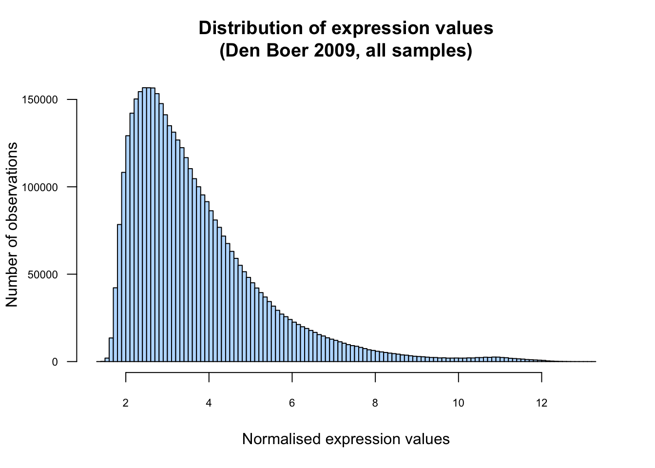
Empirical distribution of all the expression values.
Compute a table with the mean expression profile per cancer type (one row per gene, one column per cancer type) and draw them with box plots.
Sample classes
Load the pheno table. We will use the three following columns:
Sample.GEO.ID: the identifier of the sample in the Gene Expression Omnibus (GEO) database.Sample.title: cancer type of each sample.sample.labels: A short label (1 or 2 letters) for each cancer type
Count the number of samples per group and draw a barplot with the result.
Exploring the data space
The expression table contains 190 biological samples (columns) characterized by an expression profile covering 22283 genes (rows). We can thus consider that each individual (biological sample) is a point in an hyperspace with 22283 dimensions.
Highest variance genes
#### Dot plots with the genes having the highest variance ####

par(mfrow = c(2, 2))
for (i in c(1, 3, 5, 7)) {
  plot(t(exprTable[order(rowStat$var, decreasing = TRUE)[c(i, i + 1)], ]),
       panel.first = grid(),
       col = sampleColor)
  legend("topright",
         cex = 0.7,
         legend = as.vector(groupDescriptions$group.labels),
         col = as.vector(groupDescriptions$group.colors), pch = 1)
}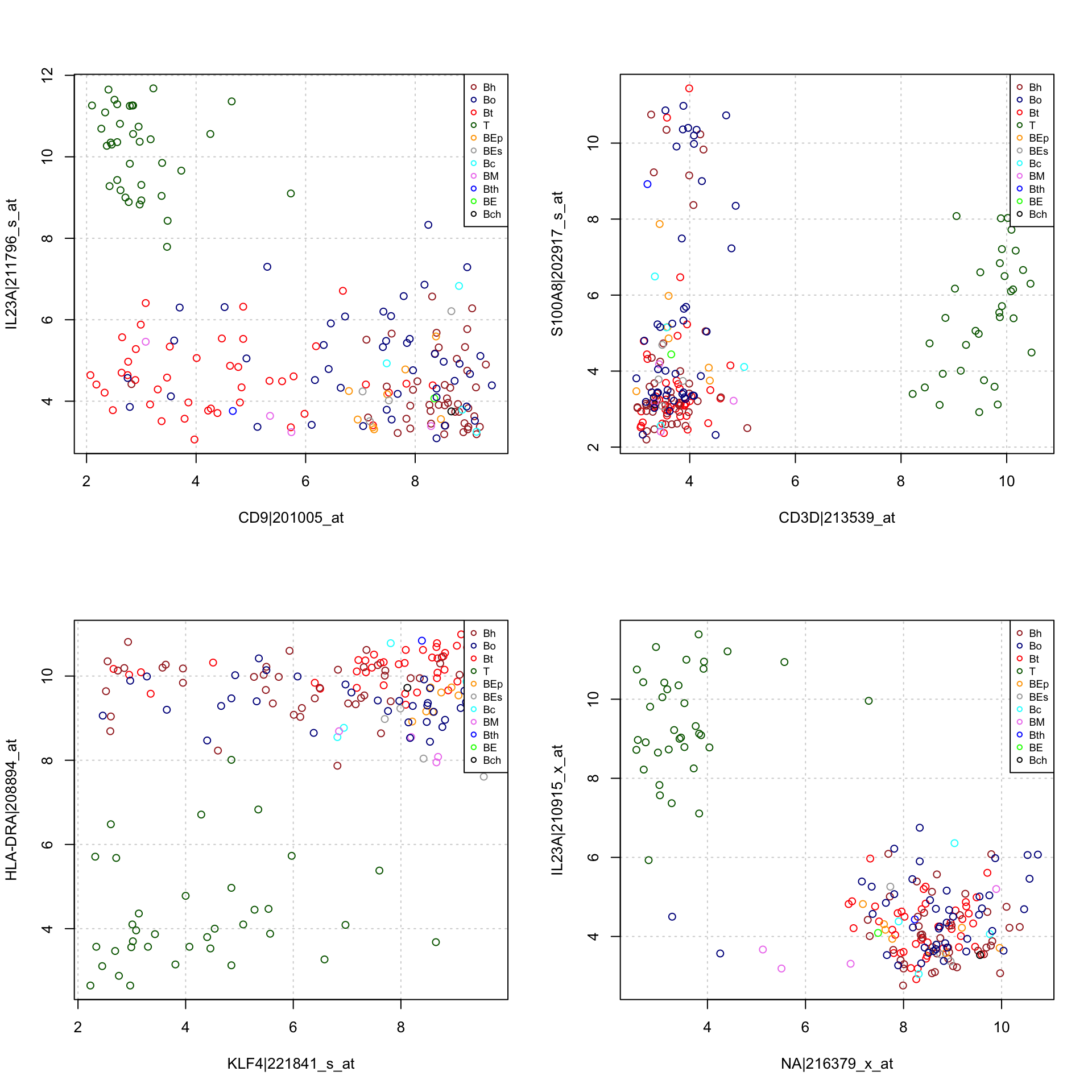
Dot plot of,the individuals on the two variables (genes) having the highest variance. Colors and letters denote the cancer subtypes.
Data reduction with Principal Component Analysis
#### Compute principal components ####
message("Computing principal components")
exprPCs <- prcomp(x = t(exprTable))
# class(exprPCs)
# attributes(exprPCs)
#### Visualise the data on the first principal components ####
par(mfrow = c(2, 2))
par(mar=c(5,4,1, 1))
## Plot the distribution of variance for the first components
plot(exprPCs, las = 1, xlab = "Components", main = NULL)
## Plot the first components with sample-wise colors and labels
plot(exprPCs$x[, c(1,2)], type = "none", las = 1, panel.first = grid())
text(exprPCs$x[, c(1,2)], col = sampleColor, labels = sampleLabel, cex = 0.8)
## Plot components 3 and 4 with sample-wise colors and labels
plot(exprPCs$x[, c(3,4)], type = "none", las = 1, panel.first = grid())
text(exprPCs$x[, c(3,4)], col = sampleColor, labels = sampleLabel, cex = 0.8)
## Plot components 5 and 6 with sample-wise colors and labels
plot(exprPCs$x[, c(5,6)], type = "none", las = 1, panel.first = grid())
text(exprPCs$x[, c(5,6)], col = sampleColor, labels = sampleLabel, cex = 0.8)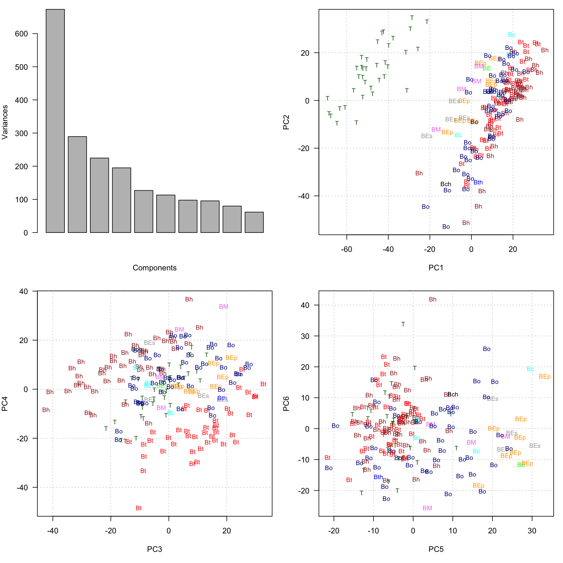
Data reduction with PCA. Topleft: variance of the first components
Saving a memory image
At the end of this tutorial, we downloaded data in tabular format (expression table, metadata, group descriptions) and loaded them in R. We will be led to re-use the same dataset for the subsequent tutorials.
For this, one possibility would be to re-run this tutorial before running the next ones. An simpler alternative is to save the content of the R memory in a file that can be reloaded in a single command.
Extract R code from this markdown
Sessiokn info
R version 3.6.1 (2019-07-05)
Platform: x86_64-apple-darwin15.6.0 (64-bit)
Running under: macOS Mojave 10.14.6

Matrix products: default
BLAS:   /Library/Frameworks/R.framework/Versions/3.6/Resources/lib/libRblas.0.dylib
LAPACK: /Library/Frameworks/R.framework/Versions/3.6/Resources/lib/libRlapack.dylib

locale:
[1] en_US.UTF-8/en_US.UTF-8/en_US.UTF-8/C/en_US.UTF-8/en_US.UTF-8

attached base packages:
[1] stats     graphics  grDevices utils     datasets  methods   base

other attached packages:
[1] knitr_1.28

loaded via a namespace (and not attached):
 [1] compiler_3.6.1  magrittr_1.5    tools_3.6.1     htmltools_0.4.0 yaml_2.2.1      Rcpp_1.0.4      stringi_1.4.6   rmarkdown_2.1   highr_0.8       stringr_1.4.0   xfun_0.12       digest_0.6.25   rlang_0.4.5     evaluate_0.14