Statistical analysis of in vitro screening for inhibitors of viral infection
Normalization and target selection methods
Franck Touret, Magali Gilles, Karine Barral, Antoine Nougaire, Etienne Decroly, Xavier de Lamballerie, and Bruno Coutard (2020). Statistical analysis by Jacques van Helden.
2020-04-20
#### Parameters ####

## Significance threshold
alpha <- 0.05

## Highlight colors
markColor <- c(
  cellCtl = "grey",
  virusCtl = "red",
  treated = "blue",
  Arbidol = "black",
  Hydroxychloroquine = "orange"
)

## Highlight point shaapes
markPCh <- c(
  cellCtl = 5,
  virusCtl = 17,
  treated = 1,
  Arbidol = 19,
  Hydroxychloroquine = 13
)
Introduction
This document describes in detail the procedure used to select molecules having a potential inhibitory effect on the infection of cultured cells by covid-19.
Pre-publication in bioRxiv:
- In vitro screening of a FDA approved chemical library reveals potential inhibitors of SARS-CoV-2 replication. Franck Touret, Magali Gilles, Karine Barral, Antoine Nougairede, Etienne Decroly, Xavier de Lamballerie, Bruno Coutard. bioRxiv 2020.04.03.023846. DOI 10.1101/2020.04.03.023846
Data
Sources
| Doc | URL |
|---|---|
| bioRxiv article | https://www.biorxiv.org/content/10.1101/2020.04.03.023846v1 |
| Supplementary tables | https://www.biorxiv.org/content/biorxiv/early/2020/04/05/2020.04.03.023846/DC1/embed/media-1.xlsx?download=true |
Supplementary data tables
#### Directories ####
message("Directories and files")

dir <- c(data = "../data",
         results = "../results",
         figures = "figures")
dir.create(dir["results"], showWarnings = FALSE, recursive = TRUE)

## Data file
supTableFile <- file.path(dir["data"], "suppl-table_Touret-2020.xlsx")
#### Load data from Excel workbook ####
message("Loading data from excel workbook.")
supTable <- read.xlsx(file = supTableFile, sheetIndex = 1)
#supTable <- read_xlsx(path = supTableFile, sheet = 1, col_names = TRUE)
# dim(supTable)
# View(supTable)
# names(supTable)
colNames <- colnames(supTable)
colNames[1] <- "ID"
colnames(supTable) <- colNames
## Suppress the last row (NA)
supTable <- supTable[!is.na(supTable$ID), ]
# dim(supTable)
## Assign row names for convenience
# View(supTable)
## Extract plate number
supTable$plateNumber <- as.numeric(substr(supTable[, 1], start = 1, stop = 2))
# table(supTable$plateNumber)
plateNumbers <- unique(supTable$plateNumber)
## Assign a color to each molecule according to its plate number
plateColor <- rainbow(n = length(plateNumbers))
names(plateColor) <- unique(supTable$plateNumber)
supTable$color <- plateColor[supTable$plateNumber]
message("\tLoaded main table with ", nrow(supTable), " rows ")The supplementary table downloaded from bioRxiv contains 1520 molecules.
Viability measurements
Cell Titer Blue intensity (CTB)
The number of viable cells per well is measured by a colorimetric test. The primary measure is the Cell Titer Blue intensity (\(CTB\)).
#### Read the CTB values from the Excel workbook ####
message("Reading Cell Titer Blue (CTB) values from file ", supTableFile)
nbPlates <- 19
rowsPerPlate <- 8
columnsPerPlate <- 12

dataPerPlate <- list()

## Control 1: uninfected cells
cellControl <- data.frame(matrix(ncol = 8, nrow = nbPlates))
colnames(cellControl) <- LETTERS[1:rowsPerPlate]

## Control 2: untreated infected cells
virusControl <- data.frame(matrix(ncol = 6, nrow = nbPlates))
colnames(virusControl) <- LETTERS[3:rowsPerPlate]

## Prepare a table to store the raw data
inhibTable <- data.frame(matrix(ncol = 8, nrow = nbPlates*rowsPerPlate * columnsPerPlate))
colnames(inhibTable) <- c("ID",
                          "Plate",
                          "Row",
                          "Column",
                          "CTB",
                          "cellControl",
                          "virusControl",
                          "Chemical.name")

i <- 2 ## for quick test
for (i in 1:nbPlates) {
  message("\tLoading data from plate ", i)
  sheetName <- paste0("Plate", i)

  ## Raw measures
  # rawMeasures <- read.xlsx(file = supTableFile,
  #                          sheetName = sheetName,
  #                          rowIndex = 30:37,
  #                          colIndex = 2:13, header = FALSE)
  rawMeasures <- read_xlsx(path = supTableFile, col_names = FALSE,
                           sheet = sheetName,
                           range = "B30:M37", progress = FALSE)
  rawMeasures <- as.data.frame(rawMeasures)
  rownames(rawMeasures) <- LETTERS[1:nrow(rawMeasures)]
  colnames(rawMeasures) <- 1:ncol(rawMeasures)
  # dim(rawMeasures)
  # View(rawMeasures)

  ## Extract control values
  cellControl[i, ] <- as.vector(rawMeasures[,1])
  virusControl[i, ] <- as.vector(rawMeasures[3:8,12])
  platevc <- mean(unlist(virusControl[i, ]))
  platecc <- mean(unlist(cellControl[i, ]))

  ## Extract all values
  r <- 1
  for (r in 1:rowsPerPlate) {
    currentRowName <- LETTERS[r]
    currentValues <- unlist(rawMeasures[currentRowName,])
    id <- paste0(sprintf("%02d",i),
                 currentRowName,
                 sprintf("%02d",1:columnsPerPlate))

    ## Compute the start index for the data table
    startIndex <- (i - 1) * (rowsPerPlate * columnsPerPlate) + (r - 1) * columnsPerPlate + 1
    # message(cat("\t\tIDs\t",  startIndex, id))
    indices <- startIndex:(startIndex + columnsPerPlate - 1)
    # length(indices)
    inhibTable[indices, "ID"] <- id
    inhibTable[indices, "Plate"] <- i
    inhibTable[indices, "Row"] <- currentRowName
    inhibTable[indices, "Column"] <- 1:columnsPerPlate
    inhibTable[indices, "CTB"] <- currentValues
    inhibTable[indices, "virusControl"] <- platevc
    inhibTable[indices, "cellControl"] <- platecc
  }

  dataPerPlate[[i]] <- list()
  dataPerPlate[[i]][["rawMeasures"]] <- rawMeasures
}

# dim(inhibTable)
# names(inhibTable)
# View(inhibTable)
# View(dataPerPlate)
# View(dataPerPlate[[1]][["rawMeasures"]])
# table(inhibTable$Row, inhibTable$Column) ## Check that there are 19 entries for each plate position

## Use the plate well ID as rowname
rownames(inhibTable) <- inhibTable$ID

## Check consistency between IDs in supplementary Touret Table 1
##  and those created here
touretIDs <- unlist(supTable$ID)
# length(touretIDs)
inhibIDs <- inhibTable$ID
# length(inhibIDs)

## Cell control: uninfected cells
cellControlIndices <- inhibTable$Column == 1
inhibTable[cellControlIndices, "Chemical.name"] <- "uninfected"

## Virus control: infected cells, no treatment
virusControlIndices <- (inhibTable$Column == 12) & (inhibTable$Row %in% LETTERS[3:8])
# table(virusControlIndices)
inhibTable[virusControlIndices, "Chemical.name"] <- "infected no treatment"

## Define the treatment type
wellType <- NA
wellType[cellControlIndices] <- "cellCtl"
wellType[virusControlIndices] <- "virusCtl"

## All the other ones are treated with a given molecule
wellType[!(virusControlIndices | cellControlIndices)] <- "treated"

inhibTable[, "wellType"] <- wellType


#### Retrieve fields from the bioRxiv supplementary Table 1 ####

for (field in c("Chemical.name",
                "Broad.Therapeutic.class",
                "Reported.therapeutic.effect",
                "Inhibition.Index")) {
  inhibTable[, field] <- NA
  inhibTable[inhibTable$ID %in% touretIDs, field] <-
    as.vector(supTable[, field])
}


# ## Retrieve the molecule names from Table 1 of the bioRxiv workbook
# inhibTable$Chemical.name <- NA
# inhibTable[inhibTable$ID %in% touretIDs, "Chemical.name"] <-
#   as.vector(supTable$Chemical.name)


kable(t(table(inhibTable$wellType)), caption = "Well types. cellCtl: no infection; virusCtl: infection without treatment; treated: inhected and treated with one molecule", )| cellCtl | treated | virusCtl |
|---|---|---|
| 152 | 1558 | 114 |
The raw data contains 19 plates with 8 rows (indiced A to H) and 12 columns (indiced from 1 to 12. )
The raw data consists of CTB measurements in cell cultures.
Distribution of raw CTB values
#### Distribution of raw measurements ####
classInterval <- 500
# xmin <- floor(min(inhibTable$CTB)/classInterval) * classInterval
xmin <- 0 ## Intently start the scale at0 to show the remnant CTB
xmax <- ceiling(max(inhibTable$CTB)/classInterval) * classInterval
breaks = seq(from = xmin, to = xmax, by = classInterval)
# range(inhibTable$CTB)

par(mfrow = c(3, 1))
par(mar = c(2,5,3,1))
hist(inhibTable[wellType == "cellCtl", "CTB"],
     main = "Uninfected (cell control)",
     xlab = "CTB",
     ylab = "Number of plate wells",
     las = 1,
     breaks = breaks, col = "palegreen", border = "palegreen")

hist(inhibTable[wellType == "virusCtl", "CTB"],
     main = "Infected, no treatment (virus control))",
     xlab = "CTB",
     ylab = "Number of plate wells",
     las = 1,
     breaks = breaks, col = "orange", border = "orange")

hist(inhibTable[wellType == "treated", "CTB"],
     main = "Treated cells",
     xlab = "CTB",
     ylab = "Number of plate wells",
     las = 1,
     breaks = breaks, col = "#AACCFF", border = "#AACCFF")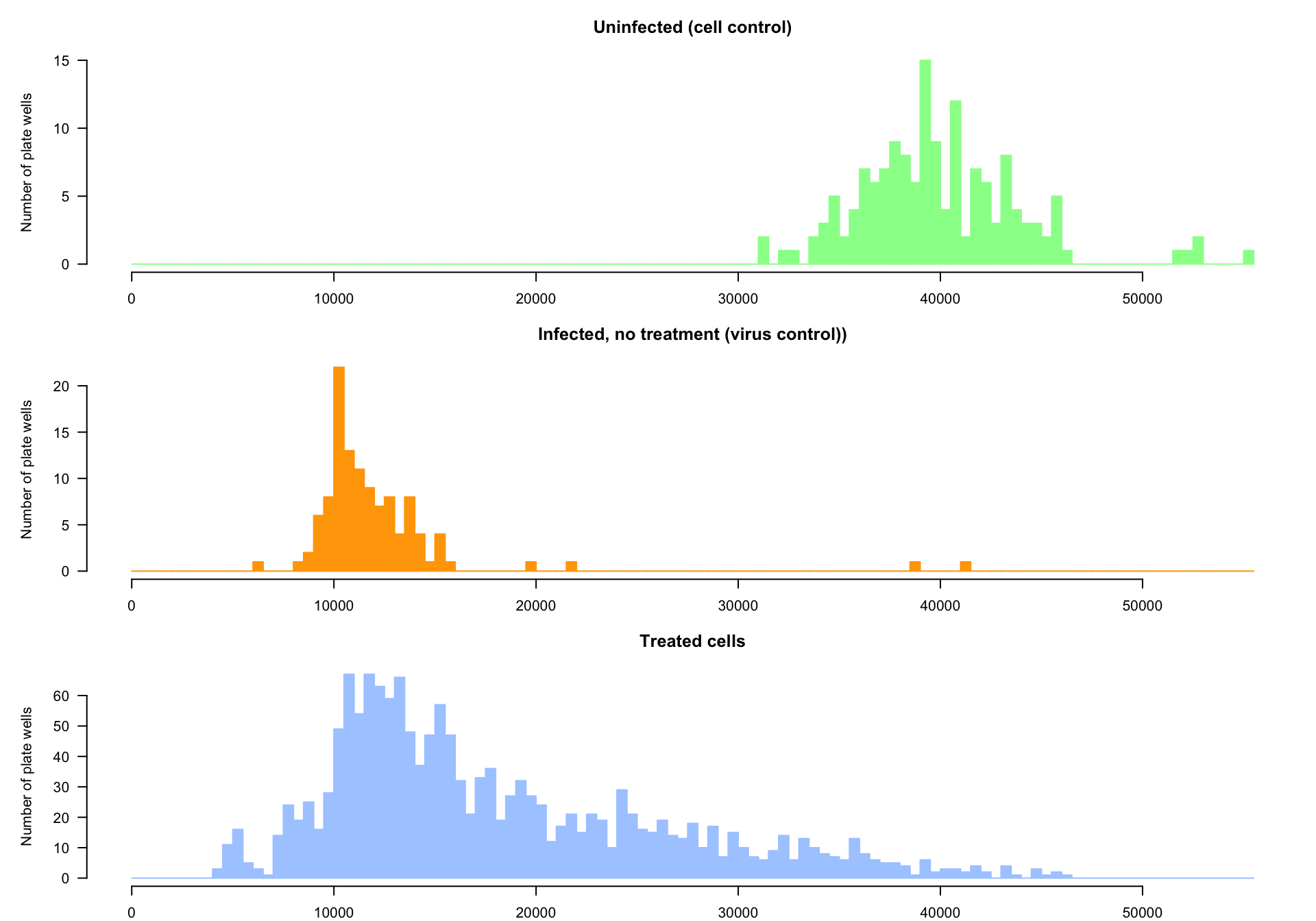
Distributions of the CTB measures. Top: uninfected cells. Middle: infected cells without treatment. Bottom: infected cells treated with a specific molecule.
Cell control.
- The top panel (green) shows the distribution of CTB measurements in controls cultures, where the cells were neither infected by the virus nor treated with a drug.
- Each plate contains 8 wells with uninfected cells (total = 152).
Virus control.
- The middle panel (orange) shows the distribution of CTB measurements in infected cells without drug treatment
- The virus control was performed on 6 wells per plate, total = 114).
Treated cells.
The bottom distribution (pale blue) shows the CTB values for cells infected and treated with a given drug.
Note that each drug was tested on a single well (no replicates). Indeed, in order to face the COVID-19 emergency, the study attempted to test as fast as possible a wide range of molecules. This first screening was thus performed without replicates. This has to be taken into account for the normalization, which should be done with no estimation of the variance for the individual drugs.
The distribution is strongly asymmetrical, and seems bi- or multi-modal. This distribution can be considered as a mixture between different distributions;
- all the drugs that have no inhibitory effect (and are thus expected to have a CTB similar to the virus control);
- various drugs that inhibit the action of the virus, each one with its specific level of inhibition. This probably corresponds to the widely dispersed values above the bulk of distribution (and above the virus control distribution)
#### Plate-wise colors ####

## Assign a color to each plate
## A trick: we alternate the colors of the rainbow in order
## to see the contrast between successive plates
platePalette <- rainbow(n = length(plateNumbers))
plateColor <- vector(length = nbPlates)
oddIndices <- seq(1, nbPlates, 2)
evenIndices <- seq(2, nbPlates, 2)
plateColor[oddIndices] <- platePalette[1:length(oddIndices)]
plateColor[evenIndices] <- platePalette[(length(oddIndices) + 1):nbPlates]
names(plateColor) <- 1:nbPlates

## Assign a color to each result according to its plate
inhibTable$color <- plateColor[inhibTable$Plate]
inhibTable$pch <- 1 # default point type for dot plots
inhibTable[inhibTable$wellType == "cellCtl", "pch"] <- markPCh["cellCtl"]
inhibTable[inhibTable$wellType == "virusCtl", "pch"] <- markPCh["virusCtl"]
# table(inhibTable$color) ## Check that each plate has 96 wells
# table(inhibTable$pch)
Arbidol treatment
A treatment with 10µM Arbidol – a broad-spectrum antiviral – was used as control, with duplicate test in 2 wells per plate.
#### Select arbidol duplicates as plate-wise milestones ####
arbidolWells <- (inhibTable$Column == 12) & (inhibTable$Row %in% c("A", "B"))
inhibTable[arbidolWells, "Chemical.name"] <- "Arbidol"
# inhibTable[arbidolWells, c("ID", "Chemical.name")]

#### Extract raw CTB measures per plate for arbidol ####
arbidoltV <- inhibTable[arbidolWells, c("Plate", "CTB")]
inhibTable[arbidolWells, "color"] <- markColor["Arbidol"]
inhibTable[arbidolWells, "pch"] <- markPCh["Arbidol"]


# table(inhibTable$color)
Hydroxychloroquine sulfate
We assin a specific label to Hydroxychloroquine sulfate, which has a specific interest since it is one of the molecules tested in an European clinical trial.
CTB boxplots
#### Boxplots per plate  ####

boxplot(CTB ~ Plate + wellType,
        main = "Cell Ttiter Blue (CTB) per plate",
        data = inhibTable,
        las = 1, col = plateColor,
        xlab = "CTB",
        cex.axis = 0.5, cex = 0.5,
        horizontal = TRUE
        )
abline(v = seq(from = 0, to = max(inhibTable$CTB), by = 2000), col = "#EEEEEE", lty = "dashed")
abline(v = seq(from = 0, to = max(inhibTable$CTB), by = 10000), col = "grey")

## Add points to denote the arbidol controls
stripchart(CTB ~ Plate, vertical = FALSE,
           data = inhibTable[arbidolWells, ],
           method = "jitter", add = TRUE, cex = 0.7,
           col = markColor["Arbidol"], pch = markPCh["Arbidol"])


legend("topright", legend = names(plateColor),
       title = "Plate", fill = plateColor, cex = 0.8)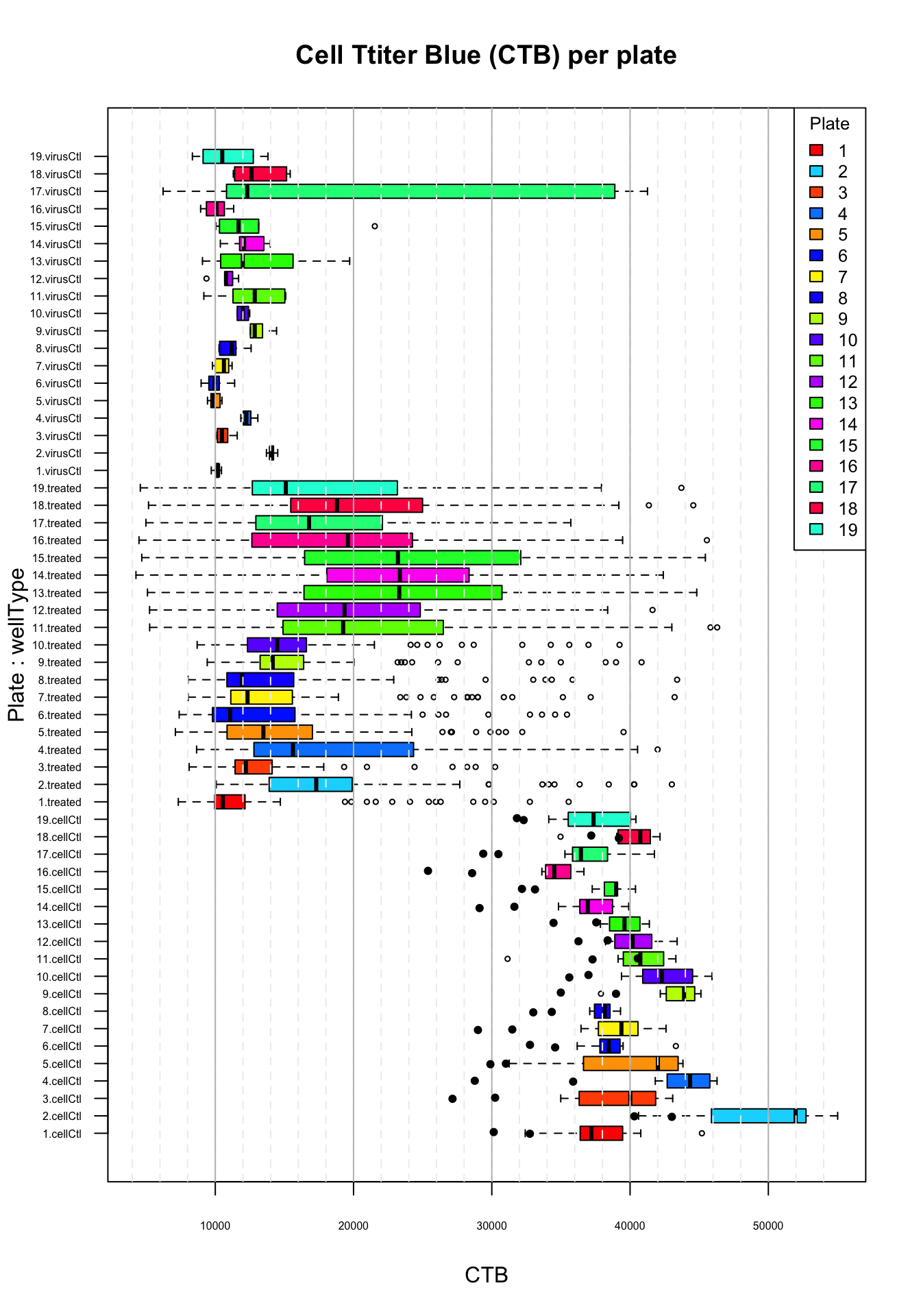
Distribution of CTB values per plate. Top virus control (untreated infected cells); middle: treated cells; bottom: cell control (uninfected). Black plain circles: arbidol control duplicates.
The boxplot of the CTB measurements highlights a plate effect, for the treated cells (middle barplots) but also for the untreated virus control (top boxplots) and uninfected cell control (bottom boxplots).
Treated:
- The medians and interquartile ranges show strong variations between plates.
- In particular, plate 1 (in red) has a the smallest median and a remarkably compact interquartile range. There are many statistical outliers (empty circles) in this plate, which might correspond to the molecules having a significant inhibitory effect.
- In contrast, plates 11 to 15 show a high median and a wide dispersion of CTB measures, and there is not a single statistical outlier.
Virus control (\(vc\))
- As expected, untreated infected cells generally gave a very small CTB, with small variations (very compact interquartile rectangles)
- There is a problem for the virus control of plate 17, which shows a broad range of values, with a third quartile falling in the range of the uninfected cells. This suggests a problem with at least 2 of the 6 replicates (missed infection ?). However, the median of the virus controls for this plate falls in the same range as for the virus control of the other plates.
Cell control (\(cc\))
- The cell control performs as expected in all the plates, with high CTB values.
- Note however that the CTB of uninfected cells show inter-plate variations, with median values ranging from ~37,000 to ~53,000.
Importantly, there is a consistency between the inter-plate differences observed for virus control, treated cells and cell control, respectively. For example, plate 2 whose consistently higher value than the other plates for the three types of wells. This highlights the importances to perform a plate-wise standardization.
Plate-wise standardization
Plate-wise control points
Taking into account the above-reported results, we apply the following procedure to standardize the individual viability measures.
For each plate, we define two control values:
- \(CTB_{cc,i}\): median CTB of the 8 cell controls (uninfected cells) of plate \(i\)
- \(CTB_{vc,i}\): median CTB of the 6 virus controls (infected untreated cells) of plate \(i\)
These two values are deliberately estimated with the median measurement of the control replicate, in order to avoid the effect of outliers as denoted for the virus control of plate 17.
#### Compute plate-wise statistics ####
plateStat <- data.frame(
  plate = plateNumbers,

  ## Mean CTB
  CTBmean = as.vector(by(
    data = inhibTable$CTB,
    INDICES = inhibTable$Plate,
    FUN = mean)),

  ## Standard deviation
  CTBsd = as.vector(by(
    data = inhibTable$CTB,
    INDICES = inhibTable$Plate,
    FUN = sd)),

  ## Median
  CTBmedian = as.vector(by(
    data = inhibTable$CTB,
    INDICES = inhibTable$Plate,
    FUN = median)),

  ## Minimum
  CTBmin = as.vector(by(
    data = inhibTable$CTB,
    INDICES = inhibTable$Plate,
    FUN = min)),

  ## maximum
 CTBmax = as.vector(by(
    data = inhibTable$CTB,
    INDICES = inhibTable$Plate,
    FUN = max)),

  # ## interquartile range
  # CTBiqr = as.vector(by(
  #   data = inhibTable$CTB,
  #   INDICES = inhibTable$Plate,
  #   FUN = IQR)),

  ## Plate-wise virus control
  CTBvc = as.vector(by(
    data = inhibTable[wellType == "virusCtl", "CTB"],
    INDICES = inhibTable[wellType == "virusCtl", "Plate"],
    FUN = median)),

  ## Plate-wise cell control
  CTBcc = as.vector(by(
    data = inhibTable[wellType == "cellCtl", "CTB"],
    INDICES = inhibTable[wellType == "cellCtl", "Plate"],
    FUN = median))

)
rownames(plateStat) <- plateStat$plate

## print the plate-wise stats in the report
kable(plateStat, caption = "Plate-wise statistics on the CTB")| plate | CTBmean | CTBsd | CTBmedian | CTBmin | CTBmax | CTBvc | CTBcc |
|---|---|---|---|---|---|---|---|
| 1 | 14968.79 | 9179.079 | 10568.5 | 7326 | 45194 | 10202.0 | 37197.5 |
| 2 | 21151.54 | 11359.022 | 17339.0 | 10069 | 55014 | 14018.0 | 51971.0 |
| 3 | 15561.16 | 8274.558 | 12261.0 | 8110 | 43083 | 10482.0 | 40016.0 |
| 4 | 20376.58 | 10986.807 | 15742.0 | 8648 | 46289 | 12241.0 | 44342.0 |
| 5 | 16882.96 | 9640.466 | 13660.5 | 7114 | 43824 | 9876.5 | 42012.0 |
| 6 | 15654.72 | 9488.589 | 11291.5 | 7389 | 43312 | 9942.0 | 38458.5 |
| 7 | 17024.33 | 9779.790 | 12338.0 | 8040 | 43221 | 10626.0 | 39375.0 |
| 8 | 16583.02 | 9286.450 | 12010.5 | 8033 | 43402 | 11185.5 | 38161.0 |
| 9 | 18603.48 | 9702.154 | 14293.5 | 9418 | 45126 | 12852.5 | 43904.5 |
| 10 | 18183.64 | 9574.292 | 14639.0 | 8690 | 45927 | 11993.0 | 42310.5 |
| 11 | 22241.27 | 10113.348 | 19335.0 | 5255 | 46301 | 12856.0 | 40742.5 |
| 12 | 21527.03 | 9444.469 | 19471.5 | 5248 | 43404 | 10781.5 | 40187.5 |
| 13 | 24039.02 | 10818.207 | 23996.5 | 5097 | 44821 | 11987.0 | 39596.5 |
| 14 | 23585.09 | 9364.788 | 23567.0 | 4263 | 42400 | 12083.0 | 36942.0 |
| 15 | 24082.91 | 10388.209 | 23327.0 | 4685 | 45445 | 11686.0 | 38995.5 |
| 16 | 19891.76 | 8991.913 | 19738.0 | 4483 | 45555 | 10090.0 | 34521.5 |
| 17 | 19518.59 | 9053.786 | 17587.0 | 4983 | 41762 | 12314.5 | 36445.0 |
| 18 | 21942.55 | 9706.601 | 19075.5 | 5173 | 44573 | 12623.0 | 40740.5 |
| 19 | 19526.67 | 9930.452 | 15299.5 | 4578 | 43712 | 10505.0 | 37360.5 |
Viability ratio and log2(ratio)
The viability ratio (\(R\)) associated to a given treatment with molecule \(m\) on a given plate \(i\) is defined as the ratio between
- the \(CTB\) measured on infected cells treated with this molecule (\(CTB_{m,i}\)) and
- the median \(CTB\) of 8 replicates of uninfected cells (denoted \(cc\) for cell control) on the same plate (\(CTB_{cc,i}\)).
\[R_{m,i} = \frac{CTB_{m,i}}{CTB_{cc, i}}\]
We further apply logarithmic transformation in order to normalise this ratio.
\[R_{m,i} = log2(R) = log2 \left( \frac{CTB_{m,i}}{CTB_{cc, i}} \right)\]
#### Compute plate-relative viability ####
inhibTable$Vratio <- inhibTable$CTB / inhibTable$CTBcc
inhibTable$Vlog2R <- log2(inhibTable$Vratio)
# table(wellType)
# hist(inhibTable[wellType == "cellCtl", "Vratio"], breaks = 50)
# hist(inhibTable[wellType == "cellCtl", "Vlog2R"], breaks = 50)

## Plate-wise virus control viability ratio
plateStat$Rvc <- as.vector(by(
  data = inhibTable[wellType == "virusCtl", "Vratio"],
  INDICES = inhibTable[wellType == "virusCtl", "Plate"],
  FUN = median))

## Plate-wise cell control viability ratio
## Note: this is 1 by definition, we compute it for validation
plateStat$Rcc <- as.vector(by(
  data = inhibTable[wellType == "cellCtl", "Vratio"],
  INDICES = inhibTable[wellType == "cellCtl", "Plate"],
  FUN = median))


## Plate-wise virus control viability log2 ratio
plateStat$Lvc <- as.vector(by(
  data = inhibTable[wellType == "virusCtl", "Vlog2R"],
  INDICES = inhibTable[wellType == "virusCtl", "Plate"],
  FUN = median))

## Plate-wise cell control viability log2 ratio
plateStat$Lcc <- as.vector(by(
  data = inhibTable[wellType == "cellCtl", "Vlog2R"],
  INDICES = inhibTable[wellType == "cellCtl", "Plate"],
  FUN = median))
Viability ratio boxplots
par(mfrow = c(1,2))


#### Boxplots of viability ratios per plate ####

Rfloor <- floor(min(inhibTable$Vratio))
Rceiling <- max(inhibTable$Vratio) * 1.1

## Box plot per plate and well type
boxplot(Vratio ~ Plate + wellType,
        main = "Viability ratio distribution",
        data = inhibTable,
        las = 1, col = plateColor,
        xlab = "R = CTB / CTBcc",
        ylim = c(min(inhibTable$Vratio), Rceiling),
        cex.axis = 0.5, cex = 0.5,
        horizontal = TRUE)
abline(v = 1, col = "#00BB00")
abline(v = seq(from = Rfloor, to = Rceiling, by = 0.05), col = "#EEEEEE", lty = "dashed")
abline(v = seq(from = Rfloor, to = Rceiling, by = 0.2), col = "grey")
legend("topright", legend = names(plateColor),
       title = "Plate", fill = plateColor, cex = 0.6)

## Add points to denote the arbidol controls
stripchart(Vratio ~ Plate, vertical = FALSE,
           data = inhibTable[arbidolWells, ],
           method = "jitter", add = TRUE, cex = 0.7,
           col = markColor["Arbidol"], pch = markPCh["Arbidol"])

legend("bottomleft",
       title = "Markers",
       legend = "Arbidol",
       col = markColor["Arbidol"],
       pch = markPCh["Arbidol"],
       cex = 0.8)


#### Boxplots of viability log(ratios) per plate ####

Lfloor <- floor(min(inhibTable$Vlog2R))
Lceiling <- ceiling(max(inhibTable$Vlog2R))

## Box plot per plate and well type
boxplot(Vlog2R ~ Plate + wellType,
        main = "Viability log2(ratio) distribution",
        data = inhibTable,
        las = 1, col = plateColor,
        xlab = "L = log2(CTB / CTBcc)",
        ylim = c(min(inhibTable$Vlog2R), Lceiling),
        cex.axis = 0.5, cex = 0.5,
        horizontal = TRUE)
abline(v = seq(from = Lfloor, to = Lceiling, by = 0.2), col = "#EEEEEE", lty = "dashed")
abline(v = seq(from = Lfloor, to = Lceiling, by = 1), col = "grey")
legend("topright", legend = names(plateColor),
       title = "Plate", fill = plateColor, cex = 0.6)

## Add points to denote the arbidol controls
stripchart(Vlog2R ~ Plate, vertical = FALSE,
           data = inhibTable[arbidolWells, ],
           method = "jitter", add = TRUE, cex = 0.7,
           col = markColor["Arbidol"], pch = markPCh["Arbidol"])

legend("bottomleft",
       title = "Markers",
       legend = "Arbidol",
       col = markColor["Arbidol"],
       pch = markPCh["Arbidol"],
       cex = 0.8)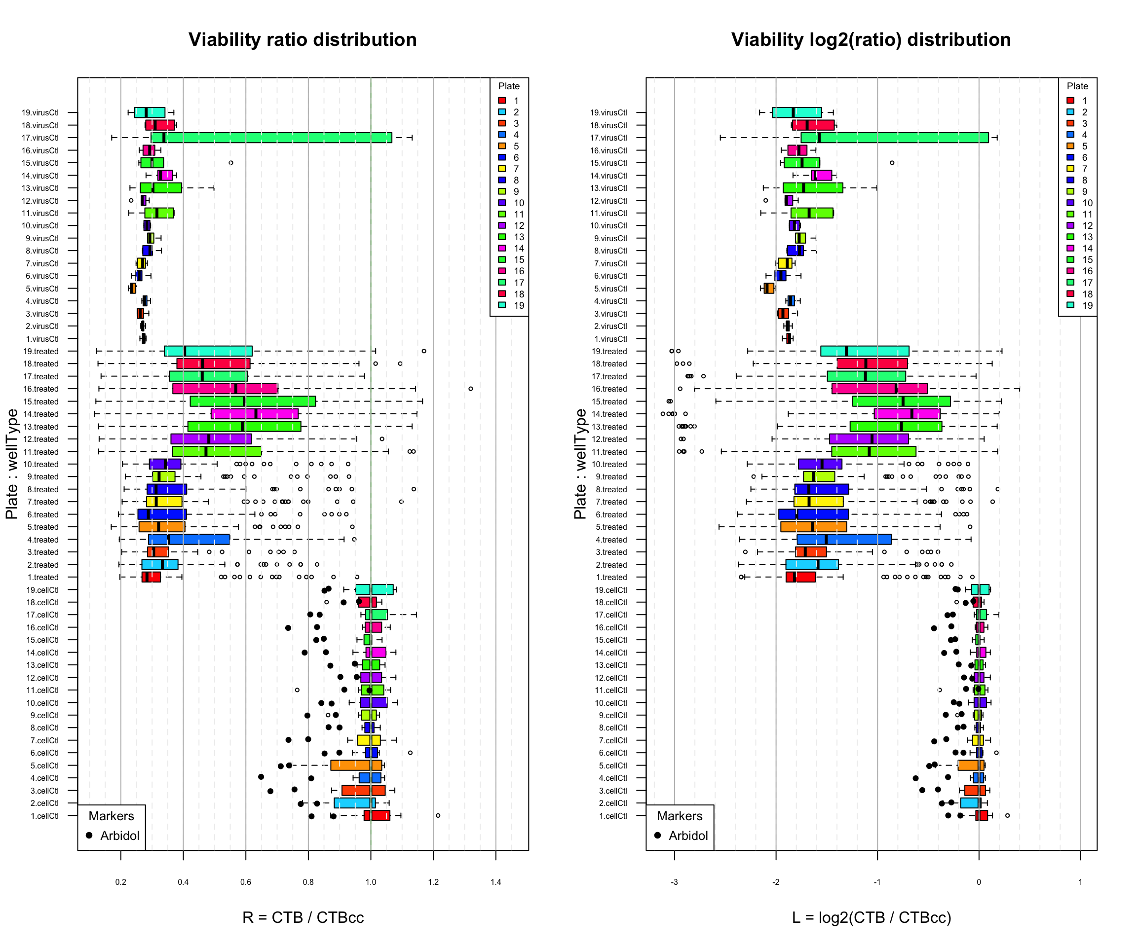
Distribution of the viability ratio (left) and log(ratio) (right) per plate. Top virus control (untreated infected cells); middle: treated cells; bottom: cell control (uninfected). Black plain circles: arbidol control duplicates.
The barplots of log2-transformed viability measures show another indication for the possible existence of a plate bias: in plates 11 to 19, several molecules are associated to a much smaller viability than in any of the untreated cells. This might reflect a cytotoxic effect of the drug that would enforce the viral infection, but there is a priori no reason to expect such effects to be concentrated on the last plates.
Two-points scaling: defining a plate-wise relative viability (\(V_{m,i}\))
A plate-wise relative viability \(V_{m,i}\) is defined to indicate the viability of cells treated with a given molecule \(m\) relative to the two controls f their plate (\(i\)):
- virus control (\(vc\)): infected untreated cells;
- cell control (\(cc\)): uninfected cells.
It is computed as follows.
\[V_{m,i} = 100 \cdot \frac{L_{m,i} - L_{vc}}{L_{cc} - L_{vc}}\]
where \(L_{cc,i}\) and \(L_{vc,i}\) denote the median values of the log2(ratios) respectively obtained in cell controls and virus controls for plate \(i\).
The plate-wise relative viability \(V_{m,i}\) is measured on a scale where
- 0 corresponds to the median of infected untreated cells (virus control), and
- 100 to the median of uninfected cells (cell control).
Note that \(V_{m,i}\) values lower than 0 denote treatments with a lower viability than the untreated virus infection. This might result from various sources: experimental flucturations, cytotoxic effect of the drug or plate bias.
\(V_{m,i}\) can also take values higher than 100, denoting a highly efficient treatment.
#### Compute relative viability from ratios ####
inhibTable$Vrel <- 100 *
  (inhibTable$Vratio - plateStat$Rvc[inhibTable$Plate]) /
    (plateStat$Rcc[inhibTable$Plate] - plateStat$Rvc[inhibTable$Plate])

#### Compute relative viability from log-ratios ####
inhibTable$Vrel <- 100 *
  (inhibTable$Vlog2R - plateStat$Lvc[inhibTable$Plate]) /
    (plateStat$Lcc[inhibTable$Plate] - plateStat$Lvc[inhibTable$Plate])

# hist(inhibTable$I, breaks = 100)
#
Relative viability boxplots
#### Boxplots of relative viability per plate ####
VrFloor = floor(min(inhibTable$Vrel))
VrCeiling = max(inhibTable$Vrel) * 1.2

## Box plot per plate and well type
boxplot(Vrel ~ Plate + wellType,
        main = "Relative viability",
        data = inhibTable,
        las = 1, col = plateColor,
        xlab = "Vr = (R - Rvc) / (Rcc - Rvc)",
        ylim = c(VrFloor, VrCeiling),
        cex.axis = 0.5, cex = 0.5,
        horizontal = TRUE)
abline(v = seq(from = VrFloor, to = VrCeiling, by = 5), col = "#EEEEEE", lty = "dashed")
abline(v = seq(from = -100, to = 150, by = 25), col = "grey")
legend("topright", legend = names(plateColor),
       title = "Plate", fill = plateColor, cex = 0.6)

## Add points to denote the arbidol controls
stripchart(Vrel ~ Plate, vertical = FALSE,
           data = inhibTable[arbidolWells, ],
           method = "jitter", add = TRUE, cex = 0.7,
           col = markColor["Arbidol"], pch = markPCh["Arbidol"])

legend("bottomleft",
       title = "Markers",
       legend = "Arbidol",
       col = markColor["Arbidol"],
       pch = markPCh["Arbidol"],
       cex = 0.8)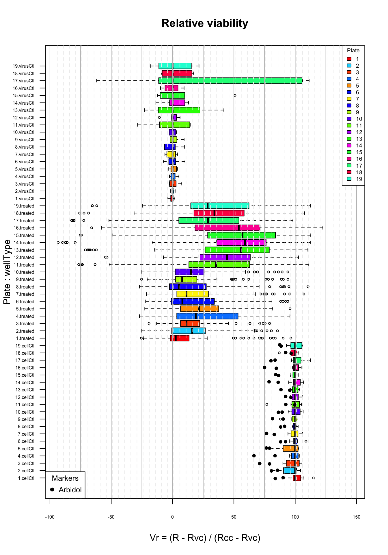
Distribution of relative viability (I) values per plate. Top virus control (untreated infected cells); middle: treated cells; bottom: cell control (uninfected). Black plain circles: arbidol control duplicates.
The box plots show that the relative viability standardises the measures by positioning each treatment relative to two milestones of its own plate:
- the median virus control (0)
- the cell control (100)
The virus controls are well regrouped in the range of smaller \(v_r\) values, except for plate 17.
The cell controls occupy the high range (their first quartile is higher than 80) and are quite compactly grouped around 100.
However, we still observe a strong difference between plates 11-19 and the other plates:
- their median is mich higher than for the plates 1 to 10;
- they also show a much wider inter-quartile rectangle, denoting a wide dispersion of values on this plate;
- for plates 11 and 13-19, this wider dispersion is even visible for the virus controls (untreated infected cells), and it is thus unlikely that it results from the particular molecules sampled on this second half of the plates.
We thus need a way to perform a between-plates standardization of the variance.
Dot plots: relative viability
#### Dot plots of the relative viability ####
VrFloor <- floor(min(inhibTable$Vrel / 10)) * 10
VrCeiling <- max(inhibTable$Vrel) * 1.1

## Virus control plots
par(mfrow = c(4,1))
plot(inhibTable[wellType == "virusCtl", "Vrel"],
     main = "Virus control (infected, untreated)",
     xlab = "Replicates, sorted per plate",
     ylab = "Vr = (R - Rvc) / (Rcc - Rvc)",
     col = inhibTable[wellType == "virusCtl", "color"],
     pch = inhibTable[wellType == "virusCtl", "pch"],
     xlim = c(0, (nbPlates * 6 * 1.05)),
     ylim = c(VrFloor, VrCeiling),
     panel.first = c(abline(h = 0, col = "red", lwd = 2),
                     abline(h = 100, col = "#008800", lwd = 2),
                     abline(h = seq(VrFloor,VrCeiling, 10), col = "#DDDDDD"),
                     abline(v = (0:19) * 6, col = "#999999")
                     ),
     xaxt = "n",
     las = 1,
     cex = 0.5
     )
mtext(plateNumbers, at = (1:19) * 6 - 3, side = 1, col = plateColor)
legend("topright",
       legend = names(plateColor),
       col = plateColor, pch = 1,
       cex = 0.7)

## Treated cells
plot(inhibTable[wellType == "treated", "Vrel"],
     main = "Relative viability (Vr)",
     xlab = "Molecules",
     ylab = "relative viability",
     col = inhibTable[wellType == "treated", "color"],
     pch = inhibTable[wellType == "treated", "pch"],
     xlim = c(0, (nbPlates * 80 * 1.05)),
     ylim = c(VrFloor, VrCeiling),
     panel.first = c(abline(h = 0, col = "red", lwd = 2),
                     abline(h = 100, col = "#008800", lwd = 2),
                     abline(h = seq(VrFloor,VrCeiling, 10), col = "#DDDDDD"),
                     abline(v = (0:19) * 80, col = "#999999")
                     ),
     xaxt = "n",
     las = 1,
     cex = 0.5
     )
mtext(plateNumbers, at = (1:19) * 80 - 40, side = 1, col = plateColor)
legend("topright",
       legend = names(plateColor),
       col = plateColor, pch = 1,
       cex = 0.6)

## Cell control
plot(inhibTable[wellType == "cellCtl", "Vrel"],
     main = "Cell control (uninfected)",
     xlab = "Replicates, sorted per plate",
     ylab = "relative viability",
     col = inhibTable[wellType == "cellCtl", "color"],
     pch = inhibTable[wellType == "cellCtl", "pch"],
     xlim = c(0, (nbPlates * 8 * 1.05)),
     ylim = c(VrFloor, VrCeiling),
     panel.first = c(abline(h = 0, col = "red", lwd = 2),
                     abline(h = 100, col = "#008800", lwd = 2),
                     abline(h = seq(VrFloor,VrCeiling, 10), col = "#DDDDDD"),
                     abline(v = (0:19) * 8, col = "#999999")
                     ),
     xaxt = "n",
     las = 1,
     cex = 0.5
     )
mtext(plateNumbers, at = (1:19) * 8 - 4, side = 1, col = plateColor)
legend("topright",
       legend = names(plateColor),
       col = plateColor, pch = 1,
       cex = 0.7)
# names(supTable)

## Rank plot
VrRank <- order(inhibTable$Vrel, decreasing = TRUE)
plot(inhibTable[VrRank, "Vrel"],
     main = "Ranked relative viability values",
     xlab = "Molecules (ranked by relative viability)",
     ylab = "relative viability",
     col = inhibTable[VrRank, "color"],
     pch = inhibTable[VrRank, "pch"],
     cex = 0.5,
     panel.first = grid(),
     xlim = c(0, length(VrRank) * 1.05)
     )
abline(h = 0, col = "red", lwd = 2)
abline(h = 100, col = "#008800", lwd = 2)
legend("topright",
       legend = names(plateColor),
       col = plateColor, pch = 1,
       cex = 0.4)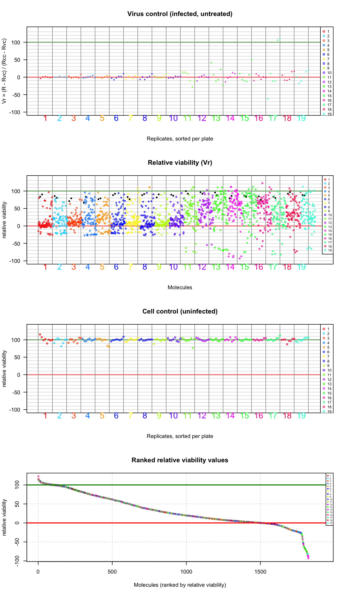
Values of the plate-wise relative viability for all the tested molecules. Molecules are colored according to the plate number. A: virus control (infected untreated); B: treated cells; C: cell control (untreated cells); D: ranked values (all types). Plain triangles: virus control (untreated infected cells). Black plain circles: arbidol control duplicates per plate. Orange square: Hydroxychloroquine sulfate.
IQR-based standardization
Plate-wise IQR-standardized viability
To take into account the between-plate differences in variance denoted above, we compute a z-scores from the original value.
- centering: substract an estimator of the plate-wise mean \(\hat{\mu}\);
- scaling: divide by an estimator of the plate-wise standard deviation (\(\hat{\sigma_i}\))
\[z_{c,i} = \frac{V_c - \hat{\mu_i}}{\hat{\sigma_i}}\]
where
- \(V_c\) is the viability for molecule \(c\);
- \(\hat{\mu_i}\) is the estimate for the mean viability of all the treated cells in plate \(i\);
- \(\hat{\sigma_i}\) is the estimate for the standard deviation of all the treated cells in plate \(i\);
In classical statistics, the estimators of centrality and dispersion are derived from the sample mean and standard deviation, respectively:
- the population mean is used as maximum likelihood estimator of the population: \(\hat{\mu} = \bar{x}\)
- the population standard deviation (\(\sigma\)) is estimated with the sample standard deviation, corrected for the systematic bias: \(\hat{\sigma} = \sqrt{n/(n-1)} \cdot s\))
However, we must be careful because each plate supposedly contain a mixture of inactive (no inhibitory effect) and active (inhibitory) molecules. The previous histograms and box plots show that these inhibitory molecules appear as statistiacal outliers (with very high viability values) and would thus strongly bias the estimation of the background variance (the variance due to fluctuations in absence of treatment).
One possibility would be to use the standard deviation of the virus control to this purpose, but this would leat to instable estimators, since they would be based on 6 points per plate. In addition, the boxplots show that the variance among treated cells is higher than the virus control, suggesting some generic effect of the treatments.
Another strategy is to consider that the variance (and standard deviation) can be estimated from the bulk of treated cell viability measures themselves, and to use robust estimators of the central tendency (i.e. the plate-wise median) and dispersion (i.e. the plate-wise interquartile range).
This approach relies on the assumption that, in each plate, the number of active molecule (statistical outliers). Since teach plate contains tests of 80 molecules, there are 19 molecules above the third quartile (\(Q3\)). However, it has to be noted that the plates were manufactured with some grouping of molecules of the same structural family. It might thus happen that some plates contain more than 19 molecules having an inhibitory effect. Such a situation would result in a loss of sensitivity, since the presence of active molecules in the inter-quartile range would lead to over-estimate the dispersion.
An alternative is to estimate the dispersion based on the range between the first quartile (\(Q1\)) and the median (\(\tilde{x}\)) of each plate.
In summary, we compute robust estimators, in order to avoid the effect of outliers (in this case, the suspected outliers are the molecules having an actual inhibitory effect). To this purpose, we use:
- the median plate-wise relative viability for all the molecules (\(\tilde{I_i}\)) to estimate the mean
- the plate-wise standardized inter-quantile range; (\(IQR_i\)) standardized by the normal \(IQR\) to estimate the standard deviation.
#### Compute plate-wise statistics ####
statPerPlate <- data.frame(
  Plate = plateNumbers,
  TrMean = as.vector(by(
    data = inhibTable[wellType == "treated", "Vrel"],
    INDICES = inhibTable[wellType == "treated", "Plate"],
    FUN = mean)),
  TrSD = as.vector(by(
    data = inhibTable[wellType == "treated", "Vrel"],
    INDICES = inhibTable[wellType == "treated", "Plate"],
    FUN = sd)),
  TrMedian = as.vector(by(
    data = inhibTable[wellType == "treated", "Vrel"],
    INDICES = inhibTable[wellType == "treated", "Plate"],
    FUN = median)),
  vcMedian = as.vector(by(
    data = inhibTable[wellType == "virusCtl", "Vrel"],
    INDICES = inhibTable[wellType == "virusCtl", "Plate"],
    FUN = median)),
  ccMedian = as.vector(by(
    data = inhibTable[wellType == "cellCtl", "Vrel"],
    INDICES = inhibTable[wellType == "cellCtl", "Plate"],
    FUN = median)),
  arbidolMean = as.vector(by(
    data = inhibTable[arbidolWells, "Vrel"],
    INDICES = inhibTable[arbidolWells, "Plate"],
    FUN = mean)),
  TrMin = as.vector(by(
    data = inhibTable[wellType == "treated", "Vrel"],
    INDICES = inhibTable[wellType == "treated", "Plate"],
    FUN = min)),
  TrMax = as.vector(by(
    data = inhibTable[wellType == "treated", "Vrel"],
    INDICES = inhibTable[wellType == "treated", "Plate"],
    FUN = max)),
  TrQ1 = as.vector(by(
    data = inhibTable[wellType == "treated", "Vrel"],
    INDICES = inhibTable[wellType == "treated", "Plate"],
    FUN = quantile, probs = 0.25)),
  TrQ3 = as.vector(by(
    data = inhibTable[wellType == "treated", "Vrel"],
    INDICES = inhibTable[wellType == "treated", "Plate"],
    FUN = quantile, probs = 0.75)),
  TrIQR = as.vector(by(    data = inhibTable[wellType == "treated", "Vrel"],
    INDICES = inhibTable[wellType == "treated", "Plate"],
    FUN = IQR))
)
rownames(statPerPlate) <- statPerPlate$Plate
We define a plate-wise scaling factor from the interquantile range, standardized by the inter-quartile range of a Gaussian distribution.
\[S_i = \frac{Q3_N - Q1_N}{Q3_i - Q3_i} = \frac{1.349}{Q3_i - Q3_i}\]
Where \(Q1\) and \(Q3\) denote the first and third quartile, \(N\) the Normal distribution, and \(i\) is the plate number.
The relative viabilities of each plate are then multiplied by the corresponding scaling factor to obtain plate-wise standardized values (\(z\)), which will have the same inter-quartile range as the normal distribution.
\[z_{c,i} = \frac{I_{m,i} - \hat{\mu_i}}{\hat{\sigma_i}} = (I_{m,i} - \tilde{I_i}) \frac{Q3_N - Q1_N}{Q3_i - Q3_i} = (v_c - \tilde{v_i}) \cdot S_i\]
where
- \(Q1_N\) and \(Q3_N\) are the first and third quartiles of the normal distribution,
- \(Q1_i\) and \(Q3_i\) are the first and third quartiles of the relative viability for all the molecules tested on plate \(i\),
The table below indicates the plate-wise statistics and scaling factor.
#### Scaling factor per plate ####

## Compute scaling factor based on the standardized inter-quartile range.
statPerPlate$scaling <-
  (qnorm(p = 0.75) - qnorm(p = 0.25)) /
  (statPerPlate$TrQ3 - statPerPlate$TrQ1)

kable(statPerPlate, caption = "Plate-wise statistics of treated cells. Column prefixes: Tr = treated cells; cc = cell control (uninfected cells); vc = virus control (infected, untreated cells). ")| Plate | TrMean | TrSD | TrMedian | vcMedian | ccMedian | arbidolMean | TrMin | TrMax | TrQ1 | TrQ3 | TrIQR | scaling |
|---|---|---|---|---|---|---|---|---|---|---|---|---|
| 1 | 12.90684 | 28.85439 | 2.589052 | 0 | 100 | 86.95038 | -25.59828 | 96.51344 | -1.7821824 | 13.16103 | 14.94322 | 0.0902737 |
| 2 | 17.39446 | 27.93057 | 16.069910 | 0 | 100 | 83.09473 | -25.25135 | 85.57929 | -0.5736503 | 26.71207 | 27.28572 | 0.0494390 |
| 3 | 16.83370 | 18.63510 | 11.395323 | 0 | 100 | 75.08391 | -19.15266 | 79.09630 | 6.5846565 | 21.89036 | 15.30570 | 0.0881358 |
| 4 | 24.81053 | 34.66755 | 18.942453 | 0 | 100 | 74.97339 | -26.98529 | 95.77630 | 3.5136062 | 51.96317 | 48.44957 | 0.0278430 |
| 5 | 23.26384 | 29.05021 | 21.490158 | 0 | 100 | 77.77693 | -22.65224 | 95.78776 | 6.7390393 | 37.13402 | 30.39498 | 0.0443816 |
| 6 | 17.43508 | 30.30878 | 8.006709 | 0 | 100 | 90.14721 | -21.90392 | 93.95942 | -0.8851005 | 33.63426 | 34.51936 | 0.0390789 |
| 7 | 21.08448 | 30.61298 | 11.384151 | 0 | 100 | 79.78517 | -21.27708 | 107.11582 | 3.6549605 | 28.72765 | 25.07269 | 0.0538027 |
| 8 | 16.67873 | 30.63601 | 5.283791 | 0 | 100 | 89.77955 | -26.97461 | 110.48853 | -2.4830636 | 27.03439 | 29.51745 | 0.0457011 |
| 9 | 16.31472 | 25.35433 | 7.863786 | 0 | 100 | 85.92780 | -25.29322 | 94.09538 | 2.5641306 | 19.27661 | 16.71248 | 0.0807169 |
| 10 | 19.42648 | 25.89632 | 14.943992 | 0 | 100 | 87.83983 | -25.54365 | 94.03011 | 2.5522727 | 25.38238 | 22.83011 | 0.0590877 |
| 11 | 35.61332 | 39.56404 | 35.389084 | 0 | 100 | 95.99690 | -76.49642 | 111.03708 | 14.4378585 | 62.68187 | 48.24401 | 0.0279616 |
| 12 | 43.11607 | 30.50020 | 44.454842 | 0 | 100 | 94.35243 | -54.72326 | 102.67258 | 22.5882232 | 63.03681 | 40.44858 | 0.0333505 |
| 13 | 45.02793 | 47.46814 | 55.760669 | 0 | 100 | 92.00095 | -71.05808 | 110.34226 | 27.3510609 | 78.39580 | 51.04474 | 0.0264274 |
| 14 | 48.84468 | 46.17014 | 58.970068 | 0 | 100 | 82.41156 | -93.22169 | 112.33839 | 35.9895577 | 76.01952 | 40.02996 | 0.0336992 |
| 15 | 49.12716 | 41.55740 | 57.064352 | 0 | 100 | 85.30208 | -75.32854 | 112.66365 | 28.9231837 | 83.82389 | 54.90071 | 0.0245713 |
| 16 | 43.91908 | 38.84888 | 53.967685 | 0 | 100 | 79.82340 | -65.94913 | 122.55003 | 18.4567483 | 71.31749 | 52.86074 | 0.0255195 |
| 17 | 26.21813 | 40.33094 | 28.927309 | 0 | 100 | 81.93965 | -82.28630 | 98.15012 | 5.1396817 | 53.96415 | 48.82447 | 0.0276292 |
| 18 | 35.81653 | 36.11849 | 34.146657 | 0 | 100 | 94.46603 | -75.77164 | 107.65872 | 17.4846896 | 58.06189 | 40.57720 | 0.0332448 |
| 19 | 35.74937 | 37.27653 | 28.621896 | 0 | 100 | 87.94144 | -65.45262 | 112.37523 | 15.1202507 | 62.11723 | 46.99698 | 0.0287035 |
#### Compute plate-wise IQR-standardized viability ####

## Centering: substract the median
## Scaling: divide by IQR
## Standardize: multiply by IQR of the normal distribution
plate <- as.vector(inhibTable$Plate)
inhibTable$z <- (inhibTable$Vrel
      - statPerPlate[plate, "TrMedian"]) * statPerPlate[plate, "scaling"]
# IQR(inhibTable$z)
# IQR(rnorm(n = 1000000))
# as.vector(by(data = inhibTable$z[wellType == "treated"], INDICES = inhibTable$Plate[wellType == "treated"], FUN = IQR))
# as.vector(by(data = inhibTable$z[wellType == "treated"], INDICES = inhibTable$Plate[wellType == "treated"], FUN = median))
### Descriptive statistics on the IQR-standardized viability ####
zstat <- data.frame(
mean = mean(inhibTable$z[wellType == "treated"]),
sd = sd(inhibTable$z[wellType == "treated"]),
IQR = IQR(inhibTable$z[wellType == "treated"]),
var = var(inhibTable$z[wellType == "treated"]),
min = min(inhibTable$z[wellType == "treated"]),
Q1 = as.vector(quantile(inhibTable$z[wellType == "treated"], probs = 0.25)),
median = median(inhibTable$z[wellType == "treated"]),
Q3 = as.vector(quantile(inhibTable$z[wellType == "treated"], probs = 0.75)),
max = max(inhibTable$z[wellType == "treated"])
)
kable(t(zstat),
col.names = "Stat",
caption = "Statistics of the plate-wise IQR-standardized viability")| Stat | |
|---|---|
| mean | 0.1656308 |
| sd | 1.4587500 |
| IQR | 1.2842621 |
| var | 2.1279515 |
| min | -5.1287479 |
| Q1 | -0.5507888 |
| median | 0.0000000 |
| Q3 | 0.7334733 |
| max | 8.4789023 |
Histograms of inter-quartile standardized viability
The histogram of plate-wise IQR-standardized viability shows a clear improvement: the median is much closer to the mode than with the raw or log-transformed II values.
#### Histograms of IQR-standardized viability ####
histBreaks = seq(from = floor(min(inhibTable$z)),
                 to = ceiling(max(inhibTable$z)), by = 0.1)

par(mfrow = c(3,1))

## Virus controls
hist(inhibTable[wellType == "virusCtl", "z"],
     main = "Virus control – IQR standardized viability",
     breaks = histBreaks,
     xlab = "Plate-wise z-score",
     col = "orange", border = "orange")
abline(v = 0)
abline(v = c(-1, 1), lty = "dotted")

## Treated cells
hist(inhibTable[wellType == "treated", "z"],
     main = "Treated cells – IQR standardized viability",
     breaks = histBreaks,
     xlab = "Plate-wise z-score",
     col = "grey", border = "grey")
abline(v = 0)
abline(v = c(-1, 1), lty = "dotted")
abline(v = mean(inhibTable[wellType == "treated", "z"]), col = "blue")
abline(v = median(inhibTable[wellType == "treated", "z"]), col = "darkgreen")
legend("topright", legend = c("mean", "median"),
       col = c("blue", "darkgreen"),
       lwd = 2)

## Cell controls
hist(inhibTable[wellType == "cellCtl", "z"],
     main = "Cell control (untreated) – IQR standardized viability",
     breaks = histBreaks,
     xlab = "Plate-wise z-score",
     col = "palegreen", border = "palegreen")
abline(v = 0)
abline(v = c(-1, 1), lty = "dotted")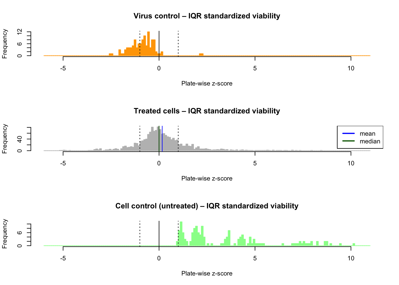
Distribution of the plate-wise IQR-standardized viability (z-scores) Top: virus control (infected, untreated); middle: treated; bottom: cell control (untreated)
Boxplots: inter-quartile standardized viability
#### Boxplots of IQR-standardized viability per plate ####

zfloor <- floor(min(inhibTable$z))
zceiling <- max(inhibTable$z) * 1.1

## Box plot per plate and well type
boxplot(z ~ Plate + wellType,
        main = "Inter-quartile standardized viability",
        data = inhibTable,
        las = 1, col = plateColor,
        xlab = "z",
        ylim = c(zfloor, zceiling),
        cex.axis = 0.5,
        cex = 0.5,
        horizontal = TRUE)
abline(v = seq(from = zfloor, to = zceiling, by = 1), col = "#EEEEEE")
abline(v = seq(from = zfloor, to = zceiling, by = 5), col = "grey")
abline(v = 0)
abline(v = c(-1, 1), lty = "dotted")
legend("topright", legend = names(plateColor),
       title = "Plate", fill = plateColor, cex = 0.6)

## Add points to denote the arbidol controls
stripchart(z ~ Plate, vertical = FALSE,
           data = inhibTable[arbidolWells, ],
           method = "jitter", add = TRUE, cex = 0.7,
           col = markColor["Arbidol"], pch = markPCh["Arbidol"])
legend("bottomleft",
       title = "Markers",
       legend = "Arbidol",
       col = markColor["Arbidol"],
       pch = markPCh["Arbidol"],
       cex = 0.8)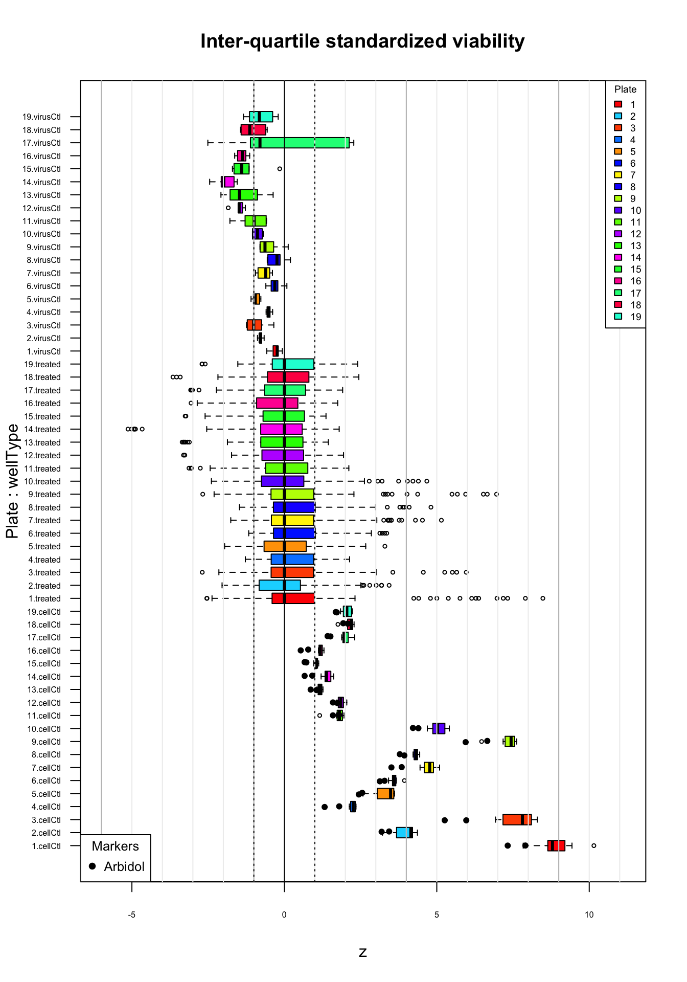
Distribution of inter-quartile standardized viability (z) values per plate. Top virus control (untreated infected cells); middle: treated cells; bottom: cell control (uninfected). Black plain circles: arbidol control duplicates.
The above boxplots show that the inter-quartile standardization efficiently corrects for the over-dispersion of the plates 11 to 19. However we may expect a lot of sensitivity for these plates. There are however still some weaknesses.
The virus control show good properties: in absence of treatment, infected cells have sligtly negative values, except for 2 outliers in plate 17.
The cell control box plots show wide variation in their medians and dispersion:
Uninfected cells (cell control) have much lower values in some plates (plates 4 and 11-19) than in other ones. This is not expected, since these cells should by definition have the same inhibition values.
Even for the plates where the cell controls have a high relative viability after IQR-based standardization, there are strong between-plates variations.
This standardization seems thus efficient to correct the apparent over-dispersion of plates 11 to 19, and thereby reduce the rate of likely false positives, but the wide between-plate variability of the untreated cells suggest that the resulting z-scores should not be interpreted as indicators of inhibition.
Dot plots: inter-quartile standardized viability
zceiling <- max(inhibTable$z) * 1.1
zRange <- c(zfloor, zceiling)

## Virus control
par(mfrow = c(4,1))
plot(inhibTable[wellType == "virusCtl", "z"],
     main = "Virus control (infected, untreated)",
     xlab = "Replicates, sorted per plate",
     ylab = "z",
     ylim = zRange,
     xlim = c(0, (19*6*1.1)),
     col = inhibTable[wellType == "virusCtl", "color"],
     pch = inhibTable[wellType == "virusCtl", "pch"],
     panel.first = c(
       abline(h = seq(from = zfloor, to = zceiling, by = 1), col = "#EEEEEE"),
       abline(h = seq(from = -5, to = zceiling, by = 5), col = "grey"),
       abline(v = (0:19) * 6, col = "#999999")
     ),
     xaxt = "n",
     cex = 0.5,
     las = 1
     )
abline(h = 0)
abline(h = c(-1, 1), lty = "dotted")
mtext(plateNumbers, at = (1:19) * 6 - 3, side = 1, col = plateColor)
legend("topright",
       legend = names(plateColor),
       col = plateColor, pch = 1,
       cex = 0.7)

## Treated cells
plot(inhibTable[wellType == "treated", "z"],
     main = "IQR-standardized viability (z)",
     xlab = "Molecules",
     ylab = "z",
     ylim = zRange,
     col = inhibTable[wellType == "treated", "color"],
     pch = inhibTable[wellType == "treated", "pch"],
     xaxt = "n",
     cex = 0.5,
     las = 1,
     xlim = c(0, length(inhibTable[wellType == "treated", "z"])*1.1)
     )
abline(h = seq(from = zfloor, to = zceiling, by = 1), col = "#EEEEEE")
abline(h = seq(from = zfloor, to = zceiling, by = 5), col = "grey")
abline(h = 0)
abline(h = c(-1, 1), lty = "dotted")
abline(v = (0:19) * 82, col = "#999999")
mtext(plateNumbers, at = (1:19) * 82 - 41, side = 1, col = plateColor)
legend("right",
       legend = names(plateColor),
       col = plateColor, pch = 1,
       cex = 0.6)
legend("topright",
       title = "Markers",
       legend = names(markColor),
       col = markColor,
       pch = markPCh,
       cex = 0.6)

## Cell control
plot(inhibTable[wellType == "cellCtl", "z"],
     panel.first = grid(),
     main = "Cell control (uninfected)",
     xlab = "Replicates, sorted per plate",
     ylab = "z",
     ylim = zRange,
     col = inhibTable[wellType == "cellCtl", "color"],
     pch = inhibTable[wellType == "cellCtl", "pch"],
     xaxt = "n",
     cex = 0.5,
     las = 1
     )
abline(h = seq(from = zfloor, to = zceiling, by = 1), col = "#EEEEEE")
abline(h = seq(from = zfloor, to = zceiling, by = 5), col = "grey")
abline(h = 0)
abline(h = c(-1, 1), lty = "dotted")
abline(v = (0:19) * 8, col = "#999999")
mtext(plateNumbers, at = (1:19) * 8 - 4, side = 1, col = plateColor)
legend("topright",
       legend = names(plateColor),
       col = plateColor, pch = 1,
       cex = 0.7)
# names(supTable)

## Rank plot
zrank <- order(inhibTable$z, decreasing = TRUE)
plot(inhibTable[zrank, "z"],
     main = "Ranked IQR-standardized viability values",
     xlab = "Molecules (ranked by z index)",
     ylab = "z",
     col = inhibTable[zrank, "color"],
     pch = inhibTable[zrank, "pch"],
     cex = 0.5, las = 1,
     panel.first = grid(),
     xlim = c(0, length(zrank) * 1.05)
     )
abline(h = seq(from = zfloor, to = zceiling, by = 1), col = "#EEEEEE")
abline(h = seq(from = zfloor, to = zceiling, by = 5), col = "grey")
abline(h = 0)
abline(h = c(-1, 1), lty = "dotted")
legend("topright",
       legend = names(plateColor),
       col = plateColor, pch = 1,
       cex = 0.4)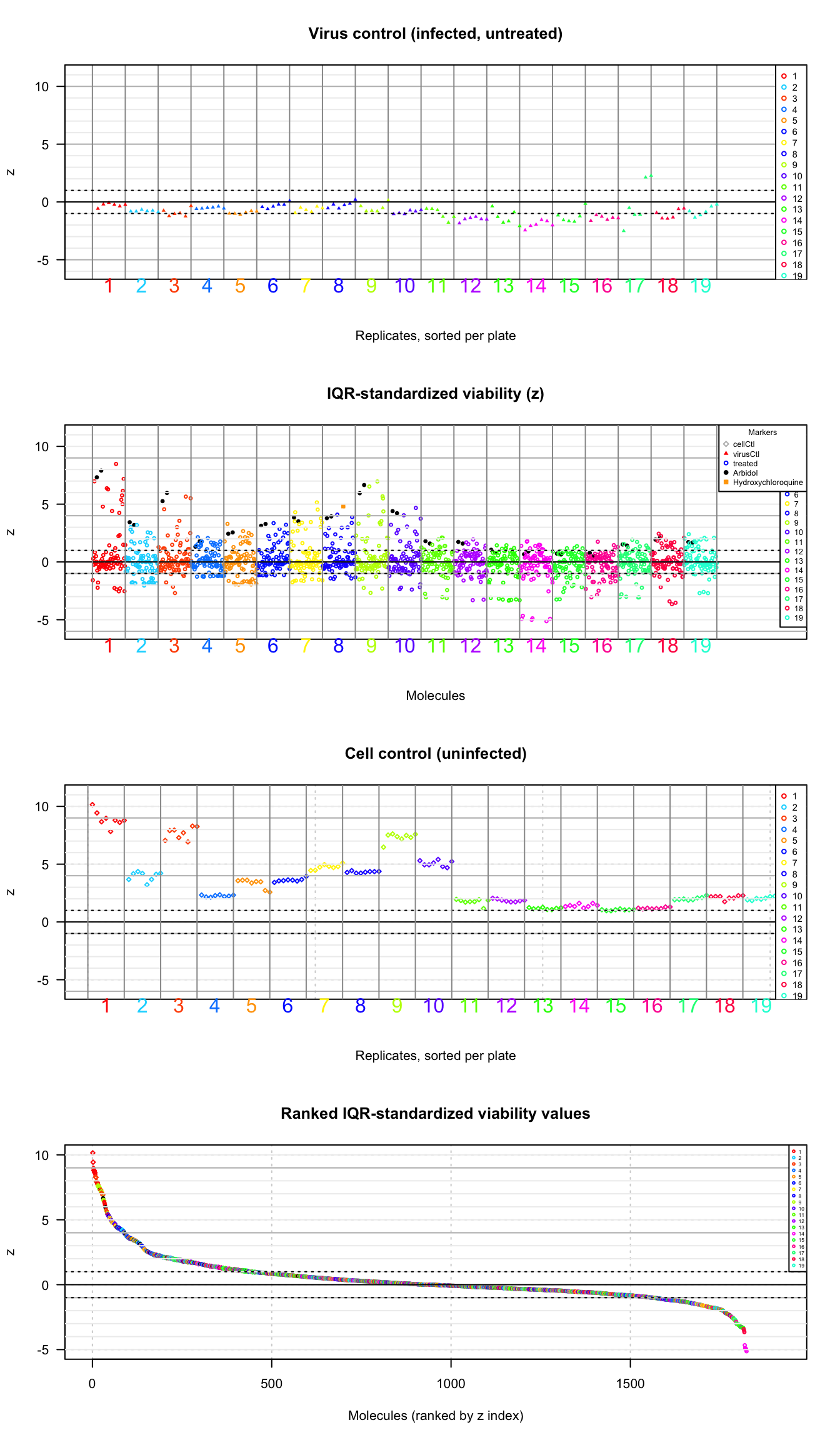
Values of the plate-wise IQR-standardized relative viability (\(z\)) for all the tested molecules. Molecules are colored according to the plate number. A: virus control (infected untreated); B: treated cells; C: cell control (untreated cells); D: ranked values (all types). Plain triangles: virus control (untreated infected cells). Black plain circles: arbidol control duplicates per plate. Orange square: Hydroxychloroquine sulfate.
The plot of IQR-standardized viability values (top panel) clearly shows that the plate-wise normalization suppressed the background bias. However it denotes a new problem: the cell controls show striking differences depending on the plates. Noticeably,they show very high values in plates 1 and 3, and very low values in plates 11 to 19, as well as in plate 4.
P-value computation
We compute the p-value as the upper tail of the normal distribution (rigth-side test) in order to detect significantly high values of the plate-wise IQR-standardized viability.
#### Compute P-value from the IQR-standardized viability ####
inhibTable$p.value <- pnorm(inhibTable$z, mean = 0, sd = 1, lower.tail = FALSE)
inhibTable$log10Pval <- log10(inhibTable$p.value)
inhibTable$e.value <- inhibTable$p.value * sum(wellType == "treated")
inhibTable$FDR <- NA
inhibTable[wellType == "treated", "FDR"] <-
  p.adjust(inhibTable[wellType == "treated", "p.value"], method = "fdr")
inhibTable$log10FDR <- log10(inhibTable$FDR)
inhibTable$sig <- -inhibTable$log10FDR
P-value histogram
hist(inhibTable[wellType == "treated", "p.value"],
     breaks = 20,
     col = "grey",
     main = "P-value histogram after plate-wise normalization",
     xlab = "Nominal P-value (unadjusted)",
     ylab = "Frequency")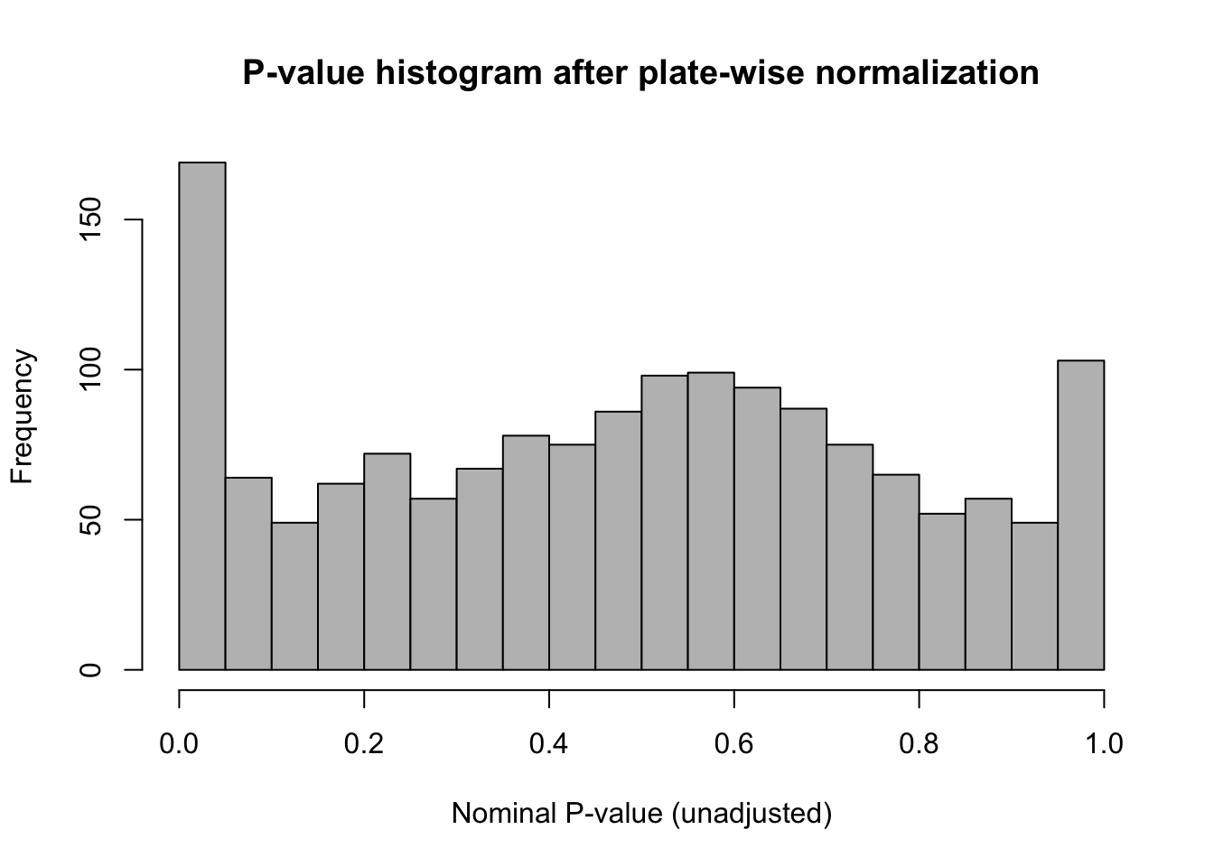
Histogram of the nominal (unadjusted) p-values derived from the plate-wise IQR-standardized relative viability.
## Estimate the proportion of tests under H0 and H1
## following the method proposed by Storey-Tibshirani (2003)
# lambda <- 0.40
# table(inhibTable[wellType == "treated", "p.value"] > lambda)
# m0 <- sum(inhibTable[wellType == "treated", "p.value"] > lambda) / (1 - lambda)
# m1 <- sum(wellType == "treated") - m0
# print(m0)
# print(m1)
#
Significance plot
#### Manhattan plot ####
sigFloor <- 0
sigCeiling <- ceiling(max(inhibTable$sig, na.rm = TRUE))

plot(x = inhibTable[wellType == "treated", "sig"],
     col = inhibTable[wellType == "treated", "color"],
     pch = inhibTable[wellType == "treated", "pch"],
     main = "Significance plot",
     xlab = "Molecules sorted per plate",
     ylab = "Significance = -log10(FDR)",
     xlim = c(0, sum(wellType == "treated") * 1.1),
     las = 1,
     xaxt = "n",
     cex = 0.5)
abline(h = 0)
abline(h = seq(0, sigCeiling, 1), lty = "dotted", col = "grey")
abline(h = -log10(alpha), col = "red")
abline(v = (0:19) * 82, col = "grey")
mtext(plateNumbers, at = (1:19) * 82 - 41, side = 1, col = plateColor)

## Legends
legend("bottomright",
       legend = names(plateColor),
       col = plateColor, pch = 1,
       cex = 0.6)
legend("topright", legend = names(markColor),
       title = "Markers",
       col = markColor,
       pch = markPCh,
       cex = 0.6)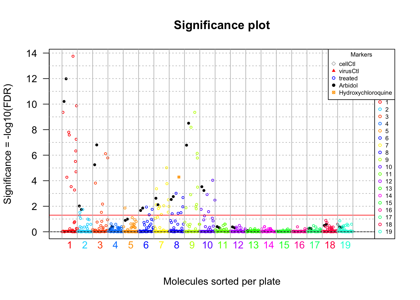
Volcano plot.
Volcano plot
#### Volcano plot ####

plot(x = inhibTable[wellType == "treated", "Vrel"],
     y = inhibTable[wellType == "treated", "sig"],
     col = inhibTable[wellType == "treated", "color"],
     pch = inhibTable[wellType == "treated", "pch"],
     main = "Volcano plot",
     xlab = "Relative viability",
     ylab = "Significance = -log10(FDR)",
     xlim = c(VrFloor, VrCeiling),
     panel.first = c(
       abline(h = seq(sigFloor, sigCeiling, 1), col = "#DDDDDD"),
       abline(v = seq(VrFloor, VrCeiling, 10), col = "#DDDDDD"),
       abline(v = seq(VrFloor, VrCeiling, 50), col = "#BBBBBB")
     ),
     las = 1,
     cex = 0.7)
abline(h = 0)
abline(h = -log10(alpha), col = "blue")
abline(v = 0, col = "red")
abline(v = 100, col = "#00BB00")
## Mark arbidol
points(x = inhibTable[arbidolWells, "Vrel"],
     y = inhibTable[arbidolWells, "sig"],
     col = inhibTable[arbidolWells, "color"],
     pch = inhibTable[arbidolWells, "pch"], cex = 0.7)
## Mark hydroxychloroquine
points(x = inhibTable[HOClSindex, "Vrel"],
     y = inhibTable[HOClSindex, "sig"],
     col = inhibTable[HOClSindex, "color"],
     pch = inhibTable[HOClSindex, "pch"], cex = 0.7)

## Legends
legend("topright",
       legend = names(plateColor),
       col = plateColor, pch = 1,
       cex = 0.7)
legend("topleft", legend = names(markColor),
       title = "Markers",
       col = markColor,
       pch = markPCh,
       cex = 0.7)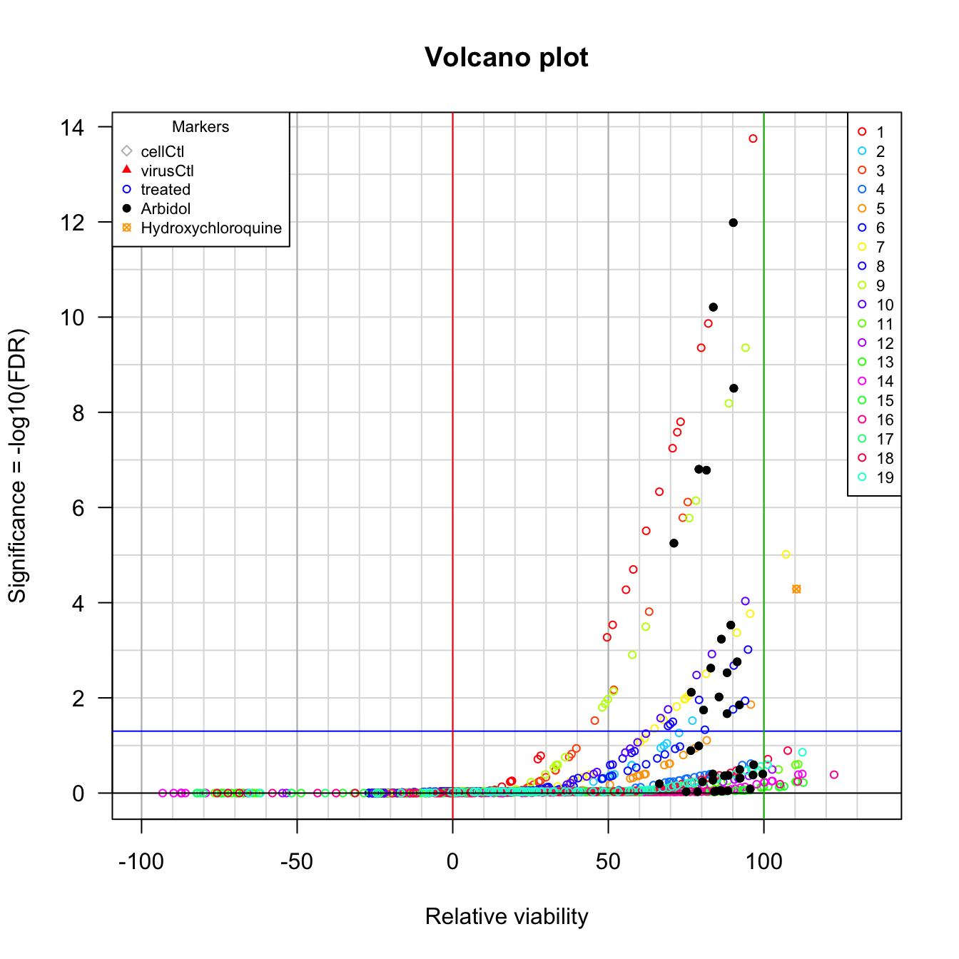
Volcano plot.
Significance of Arbidol after IQR-based standardisation
#### Relative viabilities for the arbidol contron ####
# names(inhibTable)
kable(inhibTable[arbidolWells, c("Plate", "CTB", "Vratio", "Vrel", "z", "FDR", "sig")], caption = "relative viabilities for the arbidol controls (2 replicates per plate) ")| Plate | CTB | Vratio | Vrel | z | FDR | sig | |
|---|---|---|---|---|---|---|---|
| 01A12 | 1 | 30140 | 0.8102695 | 83.73696 | 7.3255223 | 0.0000000 | 10.2090616 |
| 01B12 | 1 | 32753 | 0.8805162 | 90.16381 | 7.9056975 | 0.0000000 | 11.9838973 |
| 02A12 | 2 | 43022 | 0.8278078 | 85.57929 | 3.4364768 | 0.0095644 | 2.0193432 |
| 02B12 | 2 | 40310 | 0.7756249 | 80.61017 | 3.1908082 | 0.0179826 | 1.7451485 |
| 03A12 | 3 | 27158 | 0.6786785 | 71.07152 | 5.2596065 | 0.0000056 | 5.2500335 |
| 03B12 | 3 | 30240 | 0.7556977 | 79.09630 | 5.9668772 | 0.0000002 | 6.8041204 |
| 04A12 | 4 | 28768 | 0.6487754 | 66.39001 | 1.3210805 | 0.6399280 | 0.1938689 |
| 04B12 | 4 | 35882 | 0.8092102 | 83.55677 | 1.7990539 | 0.3966139 | 0.4016321 |
| 05A12 | 5 | 29898 | 0.7116538 | 76.50695 | 2.4417358 | 0.1279384 | 0.8929990 |
| 05B12 | 5 | 31018 | 0.7383129 | 79.04691 | 2.5544633 | 0.1022814 | 0.9902034 |
| 06A12 | 6 | 32760 | 0.8518273 | 88.15047 | 3.1319317 | 0.0214732 | 1.6681026 |
| 06B12 | 6 | 34579 | 0.8991250 | 92.14395 | 3.2879925 | 0.0140365 | 1.8527400 |
| 07A12 | 7 | 31481 | 0.7995175 | 82.92103 | 3.8488803 | 0.0023701 | 2.6252267 |
| 07B12 | 7 | 28998 | 0.7364571 | 76.64930 | 3.5114438 | 0.0076324 | 2.1173377 |
| 08A12 | 8 | 32999 | 0.8647310 | 88.15897 | 3.7874855 | 0.0029637 | 2.5281661 |
| 08B12 | 8 | 34338 | 0.8998192 | 91.40012 | 3.9356094 | 0.0017472 | 2.7576602 |
| 09A12 | 9 | 34990 | 0.7969570 | 81.53001 | 5.9461083 | 0.0000002 | 6.7837172 |
| 09B12 | 9 | 38983 | 0.8879044 | 90.32560 | 6.6560607 | 0.0000000 | 8.5044463 |
| 10A12 | 10 | 36991 | 0.8742747 | 89.35443 | 4.3967436 | 0.0002952 | 3.5299142 |
| 10B12 | 10 | 35605 | 0.8415169 | 86.32523 | 4.2177554 | 0.0005825 | 3.2347260 |
| 11A12 | 11 | 40557 | 0.9954470 | 99.62165 | 1.7960449 | 0.3966139 | 0.4016321 |
| 11B12 | 11 | 37285 | 0.9151378 | 92.37214 | 1.5933371 | 0.4843136 | 0.3148733 |
| 12A12 | 12 | 38378 | 0.9549736 | 96.50145 | 1.7357792 | 0.4170330 | 0.3798296 |
| 12B12 | 12 | 36268 | 0.9024697 | 92.20341 | 1.5924375 | 0.4843136 | 0.3148733 |
| 13A12 | 13 | 37554 | 0.9484172 | 95.58200 | 1.0523741 | 0.8170508 | 0.0877510 |
| 13B12 | 13 | 34465 | 0.8704052 | 88.41989 | 0.8630982 | 0.8917906 | 0.0497371 |
| 14A12 | 14 | 29114 | 0.7881003 | 78.69880 | 0.6648434 | 0.9330662 | 0.0300875 |
| 14B12 | 14 | 31633 | 0.8562882 | 86.12432 | 0.9150780 | 0.8732382 | 0.0588673 |
| 15A12 | 15 | 33124 | 0.8494313 | 86.49818 | 0.7232261 | 0.9199074 | 0.0362559 |
| 15B12 | 15 | 32180 | 0.8252234 | 84.10597 | 0.6644467 | 0.9330662 | 0.0300875 |
| 16A12 | 16 | 28576 | 0.8277740 | 84.63658 | 0.7826548 | 0.9060414 | 0.0428520 |
| 16B12 | 16 | 25385 | 0.7353388 | 75.01022 | 0.5369949 | 0.9330662 | 0.0300875 |
| 17A12 | 17 | 30476 | 0.8362190 | 83.61734 | 1.5110402 | 0.5361907 | 0.2706807 |
| 17B12 | 17 | 29380 | 0.8061462 | 80.26197 | 1.4183340 | 0.5798132 | 0.2367119 |
| 18A12 | 18 | 37191 | 0.9128754 | 92.23756 | 1.9312183 | 0.3203252 | 0.4944090 |
| 18B12 | 18 | 39189 | 0.9619175 | 96.69449 | 2.0793879 | 0.2549801 | 0.5934937 |
| 19A12 | 19 | 32305 | 0.8646833 | 88.54249 | 1.7199327 | 0.4239580 | 0.3726772 |
| 19B12 | 19 | 31816 | 0.8515946 | 87.34039 | 1.6854284 | 0.4339075 | 0.3626029 |
Comparison between viability scores
CTB versus viability
#### Dot plots to compare viability scores ####


# names(inhibTable)
# par(mfrow = c(2,2))

#### Dot plot: viability ratio versus relative viability ####
plot(inhibTable[, c("CTB", "Vrel")],
     main = "CTB vs relative viability",
     xlab = "Cell Titer Blue intensity (CTB)",
     ylab = "Relative viability (I)",
     col = inhibTable[, "color"],
     pch = inhibTable[, "pch"],
#     xlim = c(0, max(inhibTable$R)*1.1),
     cex = 0.5,
     las = 1)

## Mark cell controls
points(inhibTable[wellType == "cellCtl", c("CTB", "Vrel")],
       col = markColor["cellCtl"], pch = markPCh["cellCtl"], cex = 0.5)
## Mark virus controls
points(inhibTable[wellType == "virusCtl", c("CTB", "Vrel")],
       col = markColor["virusCtl"], pch = markPCh["virusCtl"], cex = 0.5)
## Mark arbidol controls
points(inhibTable[arbidolWells, c("CTB", "Vrel")],
       col = markColor["Arbidol"], pch = markPCh["Arbidol"], cex = 0.5)
## Mark Hydroxychloroquine
points(inhibTable[HOClSindex, c("CTB", "Vrel")],
       col = markColor["Hydroxychloroquine"], pch = markPCh["Hydroxychloroquine"], cex = 0.5)

## Grid + specific values for the selected metrics
abline(h = seq(from = -100, to = 150, by = 10), col = "#DDDDDD")
abline(h = 0, col = "red")
abline(h = 100, col = "#00BB00")
abline(v = seq(from = 0, to = max(inhibTable$CTB), by = 2000), col = "#DDDDDD")
abline(v = seq(from = 0, to = max(inhibTable$CTB), by = 10000), col = "#BBBBBB")
abline(v = 1)

## Legends
legend("bottomright", legend = names(plateColor),
       title = "Plate", fill = plateColor, cex = 0.6)
legend("topleft", legend = names(markColor),
       title = "Markers",
       col = markColor,
       pch = markPCh,
       cex = 0.6)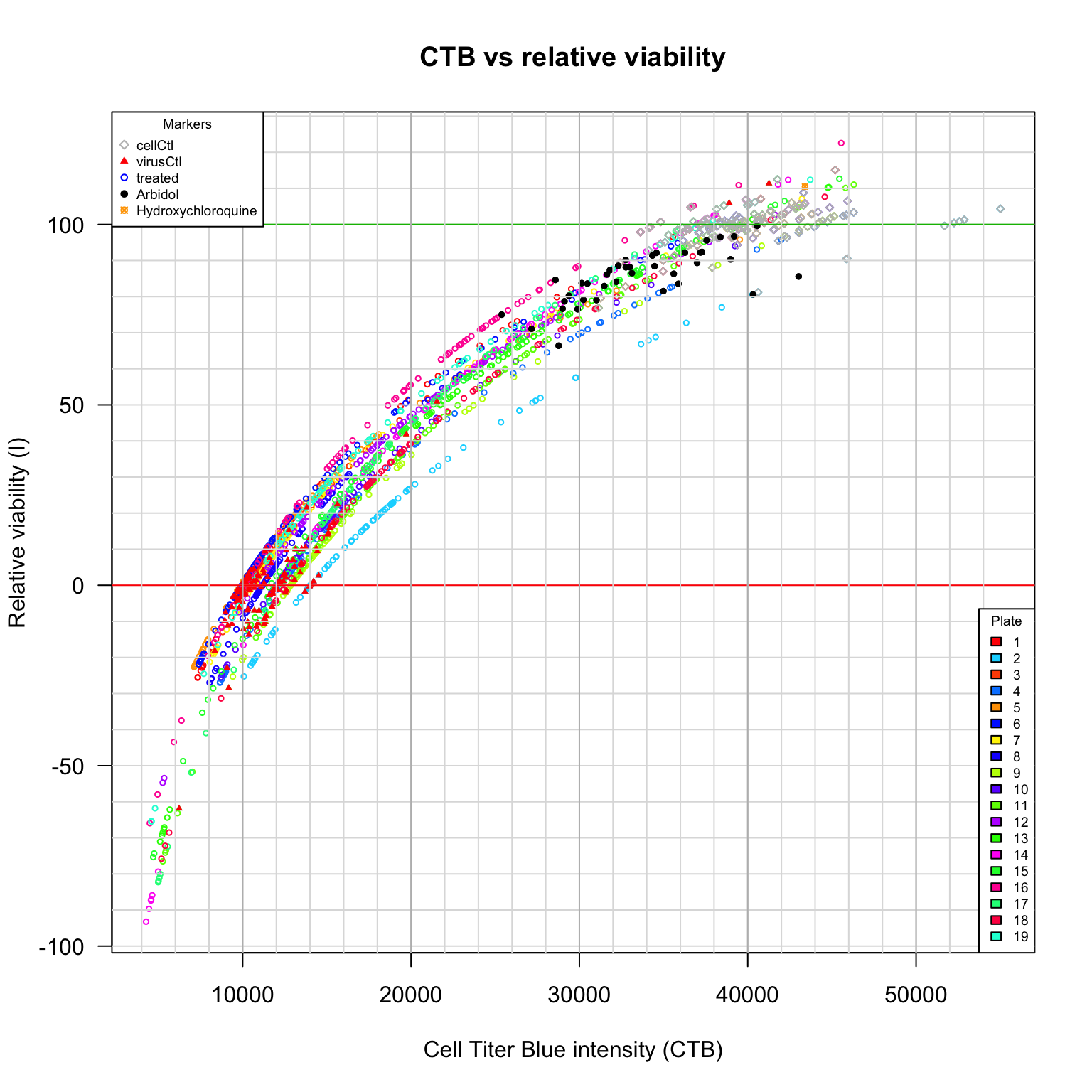
Comparison between viability scores. CTB versus relative viability (\(V_{r}\)). Diamonds: cell control (uninfected cells). Plain triangles: virus control (untreated infected cells). Black plain circles: arbidol control duplicates per plate. Orange square: Hydroxychloroquine sulfate.
Relative versus IQR-standardised viability
#### Dot plot: IQR-standardized versus relative viability ####
plot(inhibTable[, c("Vrel", "z")],
     main = "Relative viability vs IQR-standardized viability",
     xlab = "Relative viability (I)",
     ylab = "IQR-standardized viability (z-score)",
     col = inhibTable[, "color"],
     pch = inhibTable[, "pch"],
     cex = 0.5,
     xlim = c(VrFloor, VrCeiling),
     panel.first = grid(),
     las = 1)

## Mark cell controls
points(inhibTable[wellType == "cellCtl", c("Vrel", "z")],
       col = markColor["cellCtl"], pch = markPCh["cellCtl"], cex = 0.5)
## Mark virus controls
points(inhibTable[wellType == "virusCtl", c("Vrel", "z")],
       col = markColor["virusCtl"], pch = markPCh["virusCtl"], cex = 0.5)
## Mark arbidol controls
points(inhibTable[arbidolWells, c("Vrel", "z")],
       col = markColor["Arbidol"], pch = markPCh["Arbidol"], cex = 0.5)
## Mark Hydroxychloroquine
points(inhibTable[HOClSindex, c("Vrel", "z")],
       col = markColor["Hydroxychloroquine"], pch = markPCh["Hydroxychloroquine"], cex = 0.5)

## Mark milestones for the selected metrics
abline(v = seq(-100, 150, 10), col = "#EEEEEE")
abline(v = seq(-100, 150, 50), col = "#BBBBBB")
abline(v = 0, col = "red")
abline(v = 100, col = "#00BB00")
abline(h = seq(-5, 10, 1), col = "#EEEEEE")
abline(h = seq(-5, 10, 5), col = "#BBBBBB")
abline(h = 0)
abline(h = c(-1, 1), lty = "dashed")

## Legends
legend("topleft", legend = names(plateColor),
       title = "Plate", fill = plateColor, cex = 0.7)
legend("bottomright", legend = names(markColor),
       title = "Markers",
       col = markColor,
       pch = markPCh,
       cex = 0.7)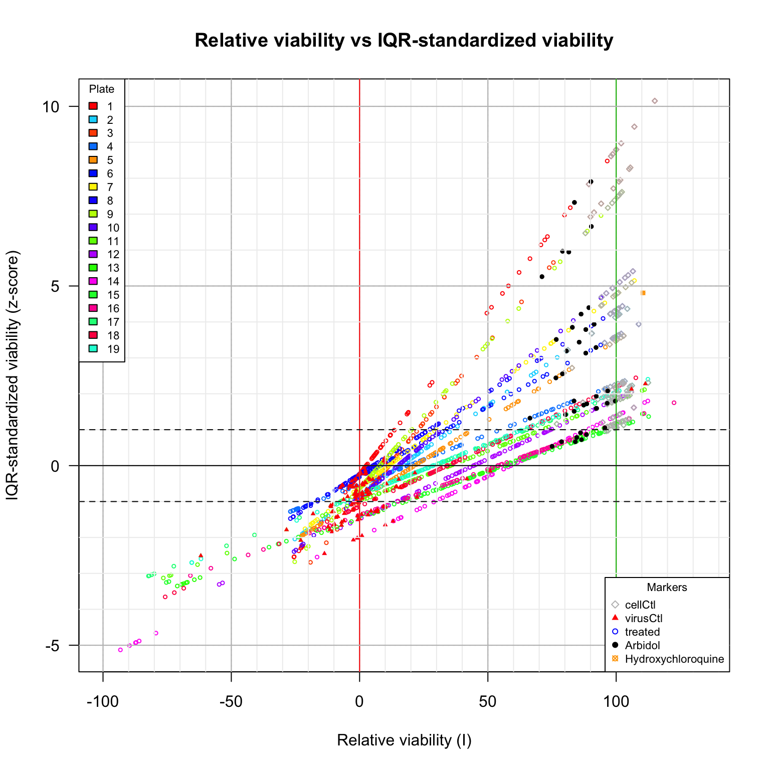
Comparison between viability scores. Relative viability versus IQR-standardized viability (z-score). Diamonds: cell control (uninfected cells). Plain triangles: virus control (untreated infected cells). Black plain circles: arbidol control duplicates per plate. Orange square: Hydroxychloroquine sulfate.
FDR versus relative viability
#### Dot plot: FDR versus relative viability ####
plot(x = inhibTable[, "Vrel"],
     y = -inhibTable[, "log10FDR"],
     main = "relative viability vs FDR",
     xlab = "relative viability",
     ylab = "-log10(FDR)",
     col = inhibTable[, "color"],
     pch = inhibTable[, "pch"],
     cex = 0.7,
     xlim = c(VrFloor, VrCeiling),
     panel.first = grid(),
     las = 1)
## Mark arbidol controls
points(x = inhibTable[arbidolWells, "Vrel"],
       y = -inhibTable[arbidolWells, "log10FDR"],
       col = markColor["Arbidol"],
       pch = markPCh["Arbidol"], cex = 0.7)
## Mark Hydroxychloroquine
points(x = inhibTable[HOClSindex, "Vrel"],
       y = -inhibTable[HOClSindex, "log10FDR"],
       col = markColor["Hydroxychloroquine"],
       pch = markPCh["Hydroxychloroquine"], cex = 0.7)

## Grid + specific values for the selected metrics
abline(v = seq(VrFloor, VrCeiling, 10), col = "#EEEEEE")
abline(v = seq(VrFloor, VrCeiling, 50), col = "#BBBBBB")
abline(v = 0, col = "red")
abline(v = 100, col = "#00BB00")
abline(h = seq(0, sigCeiling, 1), col = "#EEEEEE")
abline(h = seq(0, sigCeiling, 5), col = "#BBBBBB")
abline(h = 0)
abline(h = -log10(alpha), col = "blue", lwd = 2)

## Legends
legend("topright", legend = names(plateColor),
       title = "Plate", fill = plateColor, cex = 0.7)
legend("topleft", legend = names(markColor),
       title = "Markers",
       col = markColor,
       pch = markPCh,
       cex = 0.7)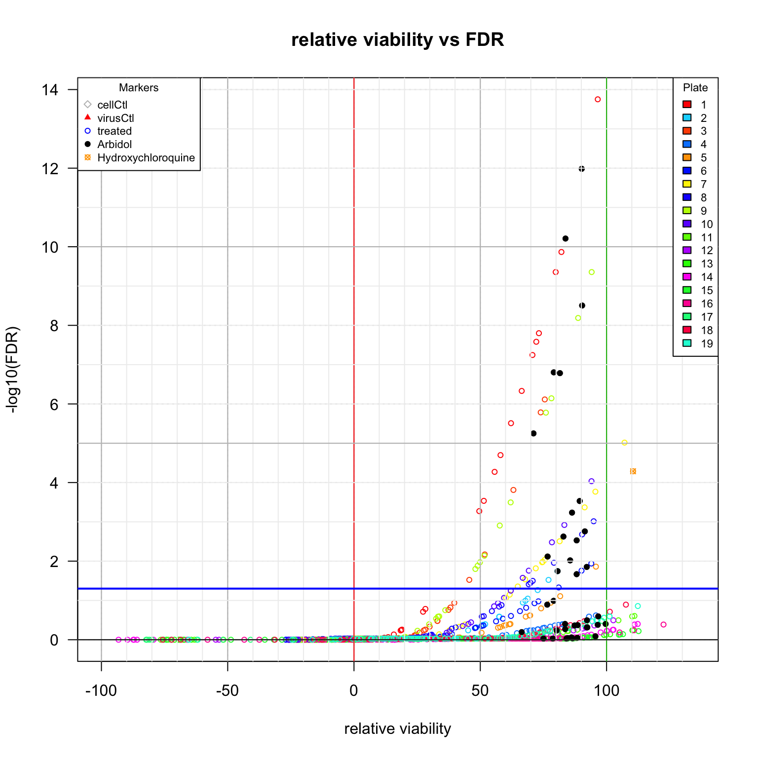
Comparison between viability scores. Diamonds: cell control (uninfected cells). Plain triangles: virus control (untreated infected cells). Black plain circles: arbidol control duplicates per plate. Orange square: Hydroxychloroquine sulfate.
Relative viability versus inhibition index
. We compare hereafter the values of the relative variability with the inhibition index defined in the bioRxiv publication (DOI 10.1101/2020.04.03.023846).
iiFloor <- floor(min(inhibTable$Inhibition.Index, na.rm = TRUE))
iiCeiling <- ceiling(max(inhibTable$Inhibition.Index, na.rm = TRUE))

#### Dot plot: Relative viability versus inhibition index ####
plot(x = inhibTable[, "Inhibition.Index"],
     y = inhibTable[, "Vrel"],
     main = "Relative viability vs inhibition index",
     xlab = "Inhibition index",
     ylab = "Vr = (R - Lvc) / (Lcc - Lvc)",
     col = inhibTable[, "color"],
     pch = inhibTable[, "pch"],
     cex = 0.5,
     xlim = c(iiFloor, iiCeiling),
     panel.first = c(
       abline(v = seq(-0.5, 2, 0.5), col = "#BBBBBB"),
       abline(h = seq(VrFloor, VrCeiling, 10), col = "#EEEEEE"),
       abline(h = seq(VrFloor, VrCeiling, 50), col = "#BBBBBB"),
       abline(h = 1)),
     las = 1)
abline(v = 1, col = "blue", lwd = 2)
abline(h = 0, col = "red")
abline(h = 100, col = "#00BB00")

## Mark Hydroxychloroquine
points(x = inhibTable[HOClSindex, "Inhibition.Index"],
       y = inhibTable[HOClSindex, "Vrel"],
       col = markColor["Hydroxychloroquine"],
       pch = markPCh["Hydroxychloroquine"], cex = 0.7)

## Legends
legend("bottomright", legend = names(plateColor),
       title = "Plate", fill = plateColor, cex = 0.7)
legend("topleft",
       title = "Markers",
       legend = "Hydroxychloroquine",
       col = markColor["Hydroxychloroquine"],
       pch = markPCh["Hydroxychloroquine"],
       cex = 0.7)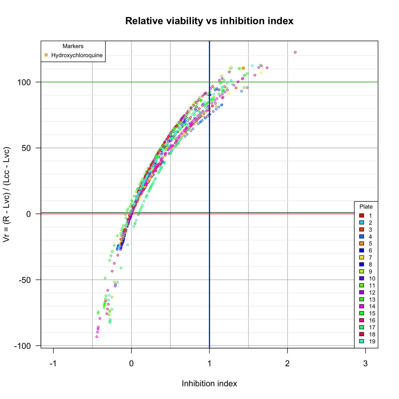
Comparison between viability scores. Diamonds: cell control (uninfected cells). Plain triangles: virus control (untreated infected cells). Black plain circles: arbidol control duplicates per plate. Orange square: Hydroxychloroquine sulfate.
Hit molecules selected by the different criteria
#### Select candidate molecules accordint to different criteria ####

## False Discovery Rate computed from the IQR-standardized viabilities
inhibTable$selected.FDR <- as.numeric(inhibTable$FDR < alpha)
# `table(inhibTable$selected.FDR)
# sum(inhibTable$selected.FDR, na.rm = TRUE)

## Previous inhibition index above 1 (Arbidol)
inhibTable$selected.ii <- as.numeric(inhibTable$Inhibition.Index >= 1)
# table(inhibTable$selected.ii)
# sum(inhibTable$selected.ii, na.rm = TRUE)

## Relative viability higher than the mean of arbidol values on the same plate
inhibTable[wellType == "treated", "selected.arbidolMean"] <- as.numeric(
  inhibTable[wellType == "treated", "Vrel"] >
    statPerPlate[inhibTable[wellType == "treated", "Plate"], "arbidolMean"])

# table(inhibTable[arbidolWells, "selected.arbidolMean"] )
# table(inhibTable[, "selected.arbidolMean"] )
# table(inhibTable[, c("selected.ii", "selected.arbidolMean")] )

# diff <- !is.na(inhibTable$selected.ii) & (inhibTable$selected.ii != inhibTable$selected.arbidolMean)
# View(inhibTable[diff, ])


kable(table(inhibTable[, c("selected.FDR", "selected.arbidolMean")]),
caption = "Contingency table of the molecules selected by different criteria. Columns: inhibition index >= 1. Rows: Vrel > arbidol mean. ")| 0 | 1 | |
|---|---|---|
| 0 | 1397 | 89 |
| 1 | 50 | 22 |
## Compute some combinations between criteria
inhibTable$selected.FDRandArbidol <-
  as.numeric(inhibTable$selected.FDR & inhibTable$selected.arbidolMean)
inhibTable$selected.FDRorArbidol <-
  as.numeric(inhibTable$selected.FDR | inhibTable$selected.arbidolMean)
inhibTable$selected.FDRonly <-
  as.numeric(inhibTable$selected.FDR & !inhibTable$selected.arbidolMean)
inhibTable$selected.ArbidolOnly <-
  as.numeric(!inhibTable$selected.FDR & inhibTable$selected.arbidolMean)


par(par.ori)
Selected hits
#### Select significant normalized II values ####

kable(t(table(inhibTable$FDR < alpha)), caption = paste("Number of tests declared positive with FDR <", alpha))| FALSE | TRUE |
|---|---|
| 1486 | 72 |
# table(inhibTable$FDR < alpha)
selected <- subset(inhibTable, inhibTable$FDR < alpha)
# names(selected)

## Sort by decreasing adjusted p-value
selected <- selected[order(selected$FDR, decreasing = FALSE), ]
# kable(names(selected), row.names=TRUE)
names(selected) <- sub(pattern = "selected.",
                       replacement = "+",
                       x = names(selected))

selectedFields <- c("ID",
                    # "CTB",
                    # "cellControl",
                    # "virusControl",
                    "Chemical.name",
                    # "Broad.Therapeutic.class",
                    "Reported.therapeutic.effect",
                    "Inhibition.Index",
                    "Vratio",
                    "Vrel",
                    "z",
                    # "p.value",
                    # "FDR",
                    "sig",
                    "+FDR",
                    "+ii",
                    "+arbidolMean",
                    "+FDRandArbidol",
                    "+FDRorArbidol",
                    "+FDRonly",
                    "+ArbidolOnly")
# kable(selectedFields)
# View(selected[ , selectedFields])

## Print selected molecules
kable(selected[ , selectedFields],
      row.names = FALSE,
      digits = 4,
caption = "Candidate moecules sorted by significance after plate-wise normalization. ")| ID | Chemical.name | Reported.therapeutic.effect | Inhibition.Index | Vratio | Vrel | z | sig | +FDR | +ii | +arbidolMean | +FDRandArbidol | +FDRorArbidol | +FDRonly | +ArbidolOnly |
|---|---|---|---|---|---|---|---|---|---|---|---|---|---|---|
| 01F08 | Benoxinate hydrochloride | Local anesthetic | 1.1929 | 0.9559 | 96.5134 | 8.4789 | 13.7518 | 1 | 1 | 1 | 1 | 1 | 0 | 0 |
| 01B12 | Arbidol | NA | NA | 0.8805 | 90.1638 | 7.9057 | 11.9839 | 1 | NA | 1 | 1 | 1 | 0 | 0 |
| 01A12 | Arbidol | NA | NA | 0.8103 | 83.7370 | 7.3255 | 10.2091 | 1 | NA | 0 | 0 | 1 | 1 | 0 |
| 01H07 | Dibucaine | Local anesthetic | 0.9095 | 0.7935 | 82.1224 | 7.1798 | 9.8665 | 1 | 0 | 0 | 0 | 1 | 1 | 0 |
| 01A06 | Atracurium besylate | Curarizing | 0.8693 | 0.7705 | 79.8475 | 6.9744 | 9.3559 | 1 | 0 | 0 | 0 | 1 | 1 | 0 |
| 09F04 | Promazine hydrochloride | Antipsychotic | 1.1610 | 0.9300 | 94.0954 | 6.9603 | 9.3559 | 1 | 1 | 1 | 1 | 1 | 0 | 0 |
| 09B12 | Arbidol | NA | NA | 0.8879 | 90.3256 | 6.6561 | 8.5044 | 1 | NA | 1 | 1 | 1 | 0 | 0 |
| 09D04 | Opipramol dihydrochloride | Antidepressant ’Antipsychotic | 1.0521 | 0.8708 | 88.7401 | 6.5281 | 8.1880 | 1 | 1 | 1 | 1 | 1 | 0 | 0 |
| 01D05 | Triamterene | Antihypertensive ’Diuretic | 0.7586 | 0.7071 | 73.2080 | 6.3750 | 7.8004 | 1 | 0 | 0 | 0 | 1 | 1 | 0 |
| 01D08 | Pyrimethamine | Antimalarial ’Antiprotozoal ’Antineoplastic | 0.7421 | 0.6977 | 72.1695 | 6.2813 | 7.5824 | 1 | 0 | 0 | 0 | 1 | 1 | 0 |
| 01H05 | Amitryptiline hydrochloride | Antidepressant | 0.7185 | 0.6841 | 70.6535 | 6.1444 | 7.2454 | 1 | 0 | 0 | 0 | 1 | 1 | 0 |
| 03B12 | Arbidol | NA | NA | 0.7557 | 79.0963 | 5.9669 | 6.8041 | 1 | NA | 1 | 1 | 1 | 0 | 0 |
| 09A12 | Arbidol | NA | NA | 0.7970 | 81.5300 | 5.9461 | 6.7837 | 1 | NA | 0 | 0 | 1 | 1 | 0 |
| 01H03 | Imipramine hydrochloride | Antidepressant | 0.6546 | 0.6475 | 66.4013 | 5.7606 | 6.3312 | 1 | 0 | 0 | 0 | 1 | 1 | 0 |
| 09G07 | Chlorcyclizine hydrochloride | Antiemetic ’Antihistaminic ’Sedative | 0.8573 | 0.7648 | 78.1773 | 5.6755 | 6.1438 | 1 | 0 | 0 | 0 | 1 | 1 | 0 |
| 03G08 | Clemizole hydrochloride | Antibacterial ’Antifungal ’Antihistaminic ’Antipruritic | 1.0073 | 0.7205 | 75.5343 | 5.6529 | 6.1147 | 1 | 1 | 1 | 1 | 1 | 0 | 0 |
| 03H10 | Orphenadrine hydrochloride | Antihistaminic ’Antiparkinsonian | 0.9732 | 0.7051 | 73.9193 | 5.5106 | 5.7855 | 1 | 0 | 0 | 0 | 1 | 1 | 0 |
| 09G08 | Diphenylpyraline hydrochloride | Antihistaminic ’Antipruritic ’Sedative | 0.8198 | 0.7444 | 75.9759 | 5.4978 | 5.7788 | 1 | 0 | 0 | 0 | 1 | 1 | 0 |
| 01G11 | Tolnaftate | Antifungal ’Antifungal | 0.5943 | 0.6129 | 62.1630 | 5.3780 | 5.5102 | 1 | 0 | 0 | 0 | 1 | 1 | 0 |
| 03A12 | Arbidol | NA | NA | 0.6787 | 71.0715 | 5.2596 | 5.2500 | 1 | NA | 0 | 0 | 1 | 1 | 0 |
| 07G07 | Pregnenolone | Anabolic ’Anti-inflammatory | 1.6589 | 1.0977 | 107.1158 | 5.1506 | 5.0163 | 1 | 1 | 1 | 1 | 1 | 0 | 0 |
| 01H04 | Sulindac | Analgesic ’Anti-inflammatory ’Antipyretic | 0.5382 | 0.5808 | 58.0051 | 5.0026 | 4.6984 | 1 | 0 | 0 | 0 | 1 | 1 | 0 |
| 08E11 | Hydroxychloroquine sulfate | Antimalarial | 1.4327 | 1.1373 | 110.4885 | 4.8080 | 4.2870 | 1 | 1 | 1 | 1 | 1 | 0 | 0 |
| 01C05 | Norethynodrel | Contraceptive | 0.5082 | 0.5636 | 55.6771 | 4.7925 | 4.2718 | 1 | 0 | 0 | 0 | 1 | 1 | 0 |
| 10G08 | Merbromin disodium salt | Antibacterial ’Antineoplastic | 1.1210 | 0.9274 | 94.0301 | 4.6730 | 4.0339 | 1 | 1 | 1 | 1 | 1 | 0 | 0 |
| 03B05 | Alverine citrate salt | Antispastic | 0.7629 | 0.6101 | 63.1168 | 4.5585 | 3.8115 | 1 | 0 | 0 | 0 | 1 | 1 | 0 |
| 07G09 | Chloroquine diphosphate | Anti-inflammatory ’Antimalarial ’Antiprotozoal | 1.3510 | 0.9436 | 95.5713 | 4.5295 | 3.7681 | 1 | 1 | 1 | 1 | 1 | 0 | 0 |
| 01E08 | Ticlopidine hydrochloride | Anticoagulant ’Antiplatelet | 0.4552 | 0.5333 | 51.4019 | 4.4065 | 3.5342 | 1 | 0 | 0 | 0 | 1 | 1 | 0 |
| 10A12 | Arbidol | NA | NA | 0.8743 | 89.3544 | 4.3967 | 3.5299 | 1 | NA | 1 | 1 | 1 | 0 | 0 |
| 09G09 | Benzethonium chloride | Antibacterial ’Antiseptic ’Antineoplastic | 0.6042 | 0.6272 | 62.0279 | 4.3720 | 3.4952 | 1 | 0 | 0 | 0 | 1 | 1 | 0 |
| 07B04 | Omeprazole | Antiulcer | 1.2487 | 0.8924 | 91.3149 | 4.3005 | 3.3683 | 1 | 1 | 1 | 1 | 1 | 0 | 0 |
| 01G06 | Diphenhydramine hydrochloride | Antiemetic ’Antihistaminic ’Antitussive ’Sedative | 0.4338 | 0.5210 | 49.6043 | 4.2442 | 3.2725 | 1 | 0 | 0 | 0 | 1 | 1 | 0 |
| 10B12 | Arbidol | NA | NA | 0.8415 | 86.3252 | 4.2178 | 3.2347 | 1 | NA | 0 | 0 | 1 | 1 | 0 |
| 08D06 | Exemestane | Antineoplastic | 1.0965 | 0.9392 | 94.8887 | 4.0950 | 3.0145 | 1 | 1 | 1 | 1 | 1 | 0 | 0 |
| 10D08 | Chlorotrianisene | Antineoplastic | 0.9163 | 0.8098 | 83.2823 | 4.0380 | 2.9208 | 1 | 0 | 0 | 0 | 1 | 1 | 0 |
| 09D02 | Dydrogesterone | Progestogen | 0.5447 | 0.5947 | 57.7090 | 4.0233 | 2.9060 | 1 | 0 | 0 | 0 | 1 | 1 | 0 |
| 08B12 | Arbidol | NA | NA | 0.8998 | 91.4001 | 3.9356 | 2.7577 | 1 | NA | 1 | 1 | 1 | 0 | 0 |
| 08H03 | Dipivefrin hydrochloride | Antiglaucoma | 1.0095 | 0.8879 | 90.3132 | 3.8859 | 2.6799 | 1 | 1 | 1 | 1 | 1 | 0 | 0 |
| 07A12 | Arbidol | NA | NA | 0.7995 | 82.9210 | 3.8489 | 2.6252 | 1 | NA | 1 | 1 | 1 | 0 | 0 |
| 08A12 | Arbidol | NA | NA | 0.8647 | 88.1590 | 3.7875 | 2.5282 | 1 | NA | 0 | 0 | 1 | 1 | 0 |
| 07H07 | Mirtazapine | Antidepressant | 1.0320 | 0.7840 | 81.4249 | 3.7684 | 2.5056 | 1 | 1 | 1 | 1 | 1 | 0 | 0 |
| 10H10 | Pridinol methanesulfonate salt | Antiparkinsonian | 0.8315 | 0.7612 | 78.3641 | 3.7474 | 2.4796 | 1 | 0 | 0 | 0 | 1 | 1 | 0 |
| 03F02 | Piroxicam | Analgesic ’Anticoagulant ’Anti-inflammatory ’Antiplatelet ’Antipyretic ’Uricosuric | 0.5726 | 0.5241 | 51.7713 | 3.5586 | 2.1704 | 1 | 0 | 0 | 0 | 1 | 1 | 0 |
| 09G04 | Famprofazone | Analgesic ’Antipyretic | 0.4661 | 0.5520 | 51.6373 | 3.5333 | 2.1386 | 1 | 0 | 0 | 0 | 1 | 1 | 0 |
| 07B03 | Nitrofural | Antibacterial ’Antidotes | 0.9359 | 0.7359 | 76.5940 | 3.5085 | 2.1173 | 1 | 0 | 0 | 0 | 1 | 1 | 0 |
| 07B12 | Arbidol | NA | NA | 0.7365 | 76.6493 | 3.5114 | 2.1173 | 1 | NA | 0 | 0 | 1 | 1 | 0 |
| 07F02 | Pirenperone | Anxiolytic | 0.9157 | 0.7258 | 75.5356 | 3.4515 | 2.0344 | 1 | 0 | 0 | 0 | 1 | 1 | 0 |
| 02A12 | Arbidol | NA | NA | 0.8278 | 85.5793 | 3.4365 | 2.0193 | 1 | NA | 1 | 1 | 1 | 0 | 0 |
| 07H10 | Tazarotene | Antipsoriatic ’Antiacneic | 0.9001 | 0.7180 | 74.7110 | 3.4072 | 1.9815 | 1 | 0 | 0 | 0 | 1 | 1 | 0 |
| 07C10 | Bromperidol | Antipsychotic | 0.8959 | 0.7159 | 74.4893 | 3.3952 | 1.9715 | 1 | 0 | 0 | 0 | 1 | 1 | 0 |
| 09F10 | Hexestrol | Antineoplastic | 0.4442 | 0.5401 | 49.8616 | 3.3899 | 1.9715 | 1 | 0 | 0 | 0 | 1 | 1 | 0 |
| 08H02 | Alendronate sodium | Antiosteoporetic | 0.8169 | 0.7743 | 79.1607 | 3.3763 | 1.9583 | 1 | 0 | 0 | 0 | 1 | 1 | 0 |
| 06D11 | Epiandrosterone | Anabolic | 1.0748 | 0.9215 | 93.9594 | 3.3589 | 1.9393 | 1 | 1 | 1 | 1 | 1 | 0 | 0 |
| 09A09 | Nilvadipine | Antianginal ’Antihypertensive | 0.4331 | 0.5341 | 48.9538 | 3.3167 | 1.8813 | 1 | 0 | 0 | 0 | 1 | 1 | 0 |
| 05A10 | Tacrine hydrochloride | CNS Stimulant | 1.4422 | 0.9408 | 95.7878 | 3.2975 | 1.8595 | 1 | 1 | 1 | 1 | 1 | 0 | 0 |
| 06B12 | Arbidol | NA | NA | 0.8991 | 92.1439 | 3.2880 | 1.8527 | 1 | NA | 1 | 1 | 1 | 0 | 0 |
| 07C03 | Biperiden hydrochloride | Antiparkinsonian ’Antineoplastic | 0.8495 | 0.6927 | 71.9731 | 3.2599 | 1.8172 | 1 | 0 | 0 | 0 | 1 | 1 | 0 |
| 09G02 | Trihexyphenidyl-D,L hydrochloride | Antiparkinsonian | 0.4224 | 0.5282 | 48.0568 | 3.2443 | 1.8009 | 1 | 0 | 0 | 0 | 1 | 1 | 0 |
| 06H02 | Vatalanib | Antineoplastic | 0.9984 | 0.8745 | 90.0896 | 3.2077 | 1.7578 | 1 | 0 | 0 | 0 | 1 | 1 | 0 |
| 10A08 | Liranaftate | Antifungal | 0.6869 | 0.6782 | 69.2049 | 3.2062 | 1.7578 | 1 | 0 | 0 | 0 | 1 | 1 | 0 |
| 02B12 | Arbidol | NA | NA | 0.7756 | 80.6102 | 3.1908 | 1.7451 | 1 | NA | 0 | 0 | 1 | 1 | 0 |
| 02C08 | Pioglitazone | NA | 0.9499 | 0.7751 | 80.5590 | 3.1883 | 1.7451 | 1 | 0 | 0 | 0 | 1 | 1 | 0 |
| 06A12 | Arbidol | NA | NA | 0.8518 | 88.1505 | 3.1319 | 1.6681 | 1 | NA | 0 | 0 | 1 | 1 | 0 |
| 10E06 | Ethoxyquin | Antifungal ’Antineoplastic | 0.6516 | 0.6579 | 66.7968 | 3.0639 | 1.5752 | 1 | 0 | 0 | 0 | 1 | 1 | 0 |
| 07H06 | Nifuroxazide | Antibacterial ’Antineoplastic | 0.7750 | 0.6554 | 67.7468 | 3.0325 | 1.5365 | 1 | 0 | 0 | 0 | 1 | 1 | 0 |
| 03E06 | Tolfenamic acid | Analgesic ’Anti-inflammatory | 0.4812 | 0.4828 | 45.6459 | 3.0187 | 1.5234 | 1 | 0 | 0 | 0 | 1 | 1 | 0 |
| 02B04 | Azacyclonol | Antipsychotic | 0.8837 | 0.7400 | 77.0208 | 3.0134 | 1.5223 | 1 | 0 | 0 | 0 | 1 | 1 | 0 |
| 08G02 | Mizolastine | Antihistaminic | 0.6881 | 0.6984 | 70.7524 | 2.9920 | 1.4982 | 1 | 0 | 0 | 0 | 1 | 1 | 0 |
| 08E07 | Rimantadine hydrochloride | Antiviral | 0.6754 | 0.6909 | 69.8764 | 2.9520 | 1.4479 | 1 | 0 | 0 | 0 | 1 | 1 | 0 |
| 08B06 | Tenatoprazole | Antiulcer | 0.6656 | 0.6851 | 69.1905 | 2.9206 | 1.4103 | 1 | 0 | 0 | 0 | 1 | 1 | 0 |
| 07D09 | Budesonide | Anti-inflammatory ’Antineoplastic | 0.7260 | 0.6309 | 64.8405 | 2.8761 | 1.3548 | 1 | 0 | 0 | 0 | 1 | 1 | 0 |
| 06F06 | Mebhydroline 1,5-naphtalenedisulfonate | Antihistaminic | 0.8344 | 0.7736 | 81.0329 | 2.8538 | 1.3303 | 1 | 0 | 0 | 0 | 1 | 1 | 0 |
Venn diagram
#### Draw a Venn diagram of the selected molecules ####

## Venn diagram
vennTable <- na.omit(inhibTable[, c("selected.FDR", "selected.arbidolMean")])
vennDiagram(object = vennTable,
            names = c(paste("FDR <", alpha),
                      paste("I >=", 1)),
            circle.col = c("#00BB00", "blue"), mar = c(0,0,0,0)
            )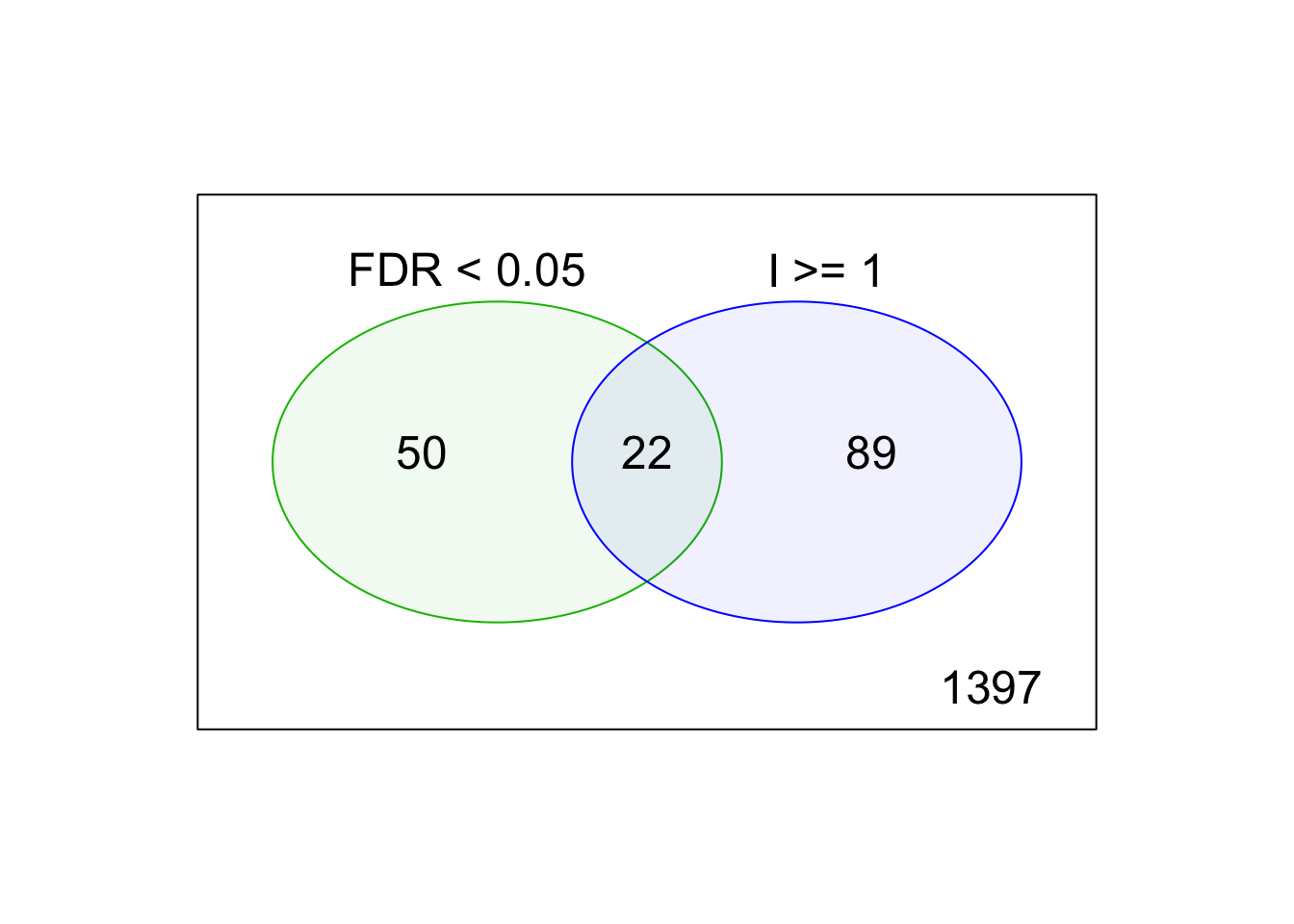
Venn diagram of the molecules selected by different criteria.
Hits per plate
#### Compute the number of candidates per plate depending on the criterion ####

## Count the number of candidates per plate for the different criteria
criteria <- c("ii", "arbidolMean", "FDR", "FDRandArbidol", "FDRorArbidol", "FDRonly", "ArbidolOnly")

# table(inhibTable$selected.ii, inhibTable$selected.arbidolMean)

candidatesPerPlate <- data.frame(matrix(
  nrow = nbPlates,
  ncol = length(criteria), 0))
row.names(candidatesPerPlate) <- 1:nbPlates
names(candidatesPerPlate) <- criteria
for (criterion in criteria) {
  candidates <- as.data.frame.table(
    table(
    subset(x = inhibTable,
           subset = inhibTable[paste0("selected.", criterion)] == 1,
           select = "Plate")))
  names(candidates) <- c("Plate", "n")
  candidatesPerPlate[as.vector(candidates$Plate), criterion] <- candidates$n
}
# apply(candidatesPerPlate, 2, sum)

ccpp <- candidatesPerPlate
ccpp["Total", ] <- apply(ccpp, 2, sum)
kable(ccpp, row.names = TRUE, ccaption = "Candidates per plate depending on the selection criteria")| ii | arbidolMean | FDR | FDRandArbidol | FDRorArbidol | FDRonly | ArbidolOnly | |
|---|---|---|---|---|---|---|---|
| 1 | 1 | 2 | 14 | 2 | 14 | 12 | 0 |
| 2 | 0 | 1 | 4 | 1 | 4 | 3 | 0 |
| 3 | 1 | 2 | 7 | 2 | 7 | 5 | 0 |
| 4 | 7 | 9 | 0 | 0 | 9 | 0 | 9 |
| 5 | 3 | 4 | 1 | 1 | 4 | 0 | 3 |
| 6 | 1 | 2 | 5 | 2 | 5 | 3 | 0 |
| 7 | 4 | 5 | 13 | 5 | 13 | 8 | 0 |
| 8 | 3 | 4 | 9 | 4 | 9 | 5 | 0 |
| 9 | 2 | 3 | 12 | 3 | 12 | 9 | 0 |
| 10 | 1 | 2 | 7 | 2 | 7 | 5 | 0 |
| 11 | 3 | 4 | 0 | 0 | 4 | 0 | 4 |
| 12 | 2 | 3 | 0 | 0 | 3 | 0 | 3 |
| 13 | 9 | 10 | 0 | 0 | 10 | 0 | 10 |
| 14 | 14 | 15 | 0 | 0 | 15 | 0 | 15 |
| 15 | 16 | 17 | 0 | 0 | 17 | 0 | 17 |
| 16 | 9 | 11 | 0 | 0 | 11 | 0 | 11 |
| 17 | 3 | 4 | 0 | 0 | 4 | 0 | 4 |
| 18 | 3 | 4 | 0 | 0 | 4 | 0 | 4 |
| 19 | 8 | 9 | 0 | 0 | 9 | 0 | 9 |
| Total | 90 | 111 | 72 | 22 | 161 | 50 | 89 |
#### Compare number of candidates per plate according to the criteria ####
names(candidatesPerPlate)
[1] "ii" "arbidolMean" "FDR" "FDRandArbidol" "FDRorArbidol" "FDRonly" "ArbidolOnly" maxc <- max(candidatesPerPlate)
plot(candidatesPerPlate[, c("FDR", "arbidolMean")],
main = "Candidates per plate",
type = "n",
xlab = paste("FDR < ", alpha),
ylab = paste("Relative viability arbidol mean"),
xlim = c(0, maxc * 1.1),
las = 1, pch = 20,
panel.first =
c(abline(h = seq(0, maxc, by = 1), col = "#DDDDDD"),
abline(h = seq(0, maxc, by = 5), col = "#BBBBBB"),
abline(v = seq(0, maxc, by = 1), col = "#EEEEEE"),
abline(v = seq(0, maxc, by = 5), col = "#BBBBBB")),
col = plateColor[rownames(candidatesPerPlate)])
text(candidatesPerPlate[, c("FDR", "arbidolMean")], rownames(candidatesPerPlate), col = plateColor)
legend("topright", legend = names(plateColor),
title = "Plate", col = plateColor, pch = 20, cex = 0.8)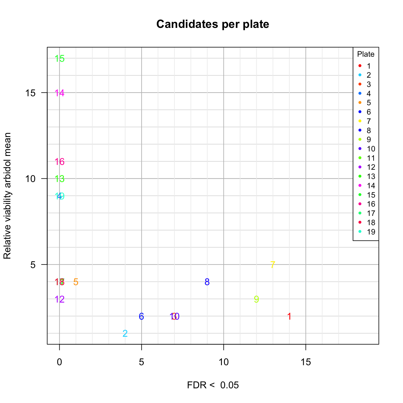
Number of candidate molecules per plate depending on the method.
Result files
#### Export result tables ####

## Define output file names
outFiles <- list(
  "All results (tsv)" =
    file.path(dir["results"], "result_table_all-molecules.tsv"),
  "All results (xlsx)" =
    file.path(dir["results"], "result_table_all-molecules.xlsx"),
  "FDR-based hits (xlsx)" =
    file.path(dir["results"], "result_table_FDR-hits.xlsx"),
  "Arbidol-based hits (xlsx)" =
    file.path(dir["results"], "result_table_arbidol-hits.xlsx"),
  "High confidence hits (xlsx)" =
    file.path(dir["results"], "result_table_HiConfidence-hits.xlsx")
)

# View(inhibTable) # check before exporting
write.table(x = inhibTable,
            file = outFiles$`All results (tsv)`,
            sep = "\t", quote = FALSE,
            row.names = FALSE, col.names = TRUE)

write.xlsx2(x = inhibTable,
            file = outFiles$`All results (xlsx)`,
            row.names = FALSE, col.names = TRUE)

# table(!is.na(inhibTable$selected.FDR) & (inhibTable$selected.FDR == 1))
# View(inhibTable[!is.na(inhibTable$selected.FDR) & (inhibTable$selected.FDR == 1), ]) # check before exporting
write.xlsx2(x = inhibTable[!is.na(inhibTable$selected.FDR) & (inhibTable$selected.FDR == 1), ],
            file = outFiles$`FDR-based hits (xlsx)`,
            row.names = FALSE, col.names = TRUE)

# View(inhibTable[!is.na(inhibTable$selected.FDR) & (inhibTable$selected.arbidolMean), ])
write.xlsx2(x = inhibTable[!is.na(inhibTable$selected.FDR) & (inhibTable$selected.arbidolMean), ],
            file = outFiles$`Arbidol-based hits (xlsx)`,
            row.names = FALSE, col.names = TRUE)

# View(inhibTable[!is.na(inhibTable$selected.FDR) & (inhibTable$selected.FDRandArbidol), ])
write.xlsx2(x = inhibTable[!is.na(inhibTable$selected.FDR) & (inhibTable$selected.FDRandArbidol), ],
            file = outFiles$`High confidence hits (xlsx)`,
            row.names = FALSE, col.names = TRUE)

# system(paste("open", dir["results"]))

## Prepare a data frame with the relative links to output files
fileLinks <- data.frame(
  name = names(outFiles),
  path = unlist(outFiles),
  basename = basename(unlist(outFiles))
)

fileLinks$link <- paste0("<a href='", fileLinks$path, "'>", fileLinks$basename, "</a>")

kable(fileLinks[, c("name", "link")], row.names = FALSE, caption = "Links to the result tables. ")| name | link |
|---|---|
| All results (tsv) | result_table_all-molecules.tsv |
| All results (xlsx) | result_table_all-molecules.xlsx |
| FDR-based hits (xlsx) | result_table_FDR-hits.xlsx |
| Arbidol-based hits (xlsx) | result_table_arbidol-hits.xlsx |
| High confidence hits (xlsx) | result_table_HiConfidence-hits.xlsx |
Libraries and versions
For the sake of reproducibility, we list hereafter the R libraries used to generate this report, as well as their versions.
R version 3.6.1 (2019-07-05)
Platform: x86_64-apple-darwin15.6.0 (64-bit)
Running under: macOS Mojave 10.14.6

Matrix products: default
BLAS:   /Library/Frameworks/R.framework/Versions/3.6/Resources/lib/libRblas.0.dylib
LAPACK: /Library/Frameworks/R.framework/Versions/3.6/Resources/lib/libRlapack.dylib

locale:
[1] en_US.UTF-8/en_US.UTF-8/en_US.UTF-8/C/en_US.UTF-8/en_US.UTF-8

attached base packages:
[1] grid      stats     graphics  grDevices utils     datasets  methods   base

other attached packages:
 [1] vioplot_0.3.4       zoo_1.8-7           sm_2.2-5.6          fitdistrplus_1.0-14 npsurv_0.4-0        lsei_1.2-0          survival_3.1-11     MASS_7.3-51.5       limma_3.40.6        VennDiagram_1.6.20  futile.logger_1.4.3 knitr_1.28          readxl_1.3.1        xlsx_0.6.3

loaded via a namespace (and not attached):
 [1] Rcpp_1.0.4           highr_0.8            pillar_1.4.3         cellranger_1.1.0     compiler_3.6.1       formatR_1.7          futile.options_1.0.1 tools_3.6.1          digest_0.6.25        evaluate_0.14        tibble_3.0.0         lifecycle_0.2.0      lattice_0.20-40      pkgconfig_2.0.3
[15] rlang_0.4.5          Matrix_1.2-18        cli_2.0.2            yaml_2.2.1           xfun_0.12            rJava_0.9-12         stringr_1.4.0        vctrs_0.2.4          xlsxjars_0.6.1       glue_1.3.2           rematch_1.0.1        fansi_0.4.1          tcltk_3.6.1          rmarkdown_2.1
[29] lambda.r_1.2.4       magrittr_1.5         htmltools_0.4.0      ellipsis_0.3.0       splines_3.6.1        assertthat_0.2.1     stringi_1.4.6        crayon_1.3.4