Using BLAST on the command line
Jacques van Helden
Created: 8/10/2018; last update: 2018-10-26
Modifications récentes
2028-20-26: dans la section “Identifying aspartokinase homologs in the proteome of interest”,
- ajout d’un seuil sur la e-value
- ajouts de liens vers Uniprot et BioCyc pour donner des clés d’interprétation
2028-20-26: ajout d’une section Counting the number of hits per protein
Course home page
This practical is part of a series of tutorials Using the resources of the IFB National Network of Ccomputing Resources (NNCR), available at https://jvanheld.github.io/using_IFB_NNCR/
Prerequisite
This practical assumes that you are connected to a cluster of the IFB NNCR. This enables you to benefit from a software environment with pre-installed software tools for the different fields of bioinformatics.
To open a connection to the IFB NNCR, follow the totirla Tutorial |
Resources
| Resource | URL and description |
|---|---|
| Ensembl Bacteria | https://bacteria.ensembl.org/index.html Database and browser for bacterial and archaeal genomes maintained at the European Bioinformatics Institute (EBI) |
| GTF format | https://genome.ucsc.edu/FAQ/FAQformat.html#format4 Specification of the Gene Transfer Format (GTF) on the UCSC genome browser Web site |
| Ensembl Bacteria Metadata | ftp://ftp.ensemblgenomes.org/pub/release-41/bacteria/species_EnsemblBacteria.txt table with information about each sequenced genome |
| Selected genomes | MICROME genome table A table containing 80 genomes of interest for the MICROME European network. |
Tutorial
Browsing genomes with EnsemblGenomes
As reference genome, we will use the strain K12 MG1655 of Escherichia coli.
In a web browser, open a connexion to Ensembl Bacteria (https://bacteria.ensembl.org).
In the Search for a genome box, type MG1655. The interface will display a list of the genomes matching this string. Select the strain with taxonomic ID (TAXID) 511145.

EnsemblGenomes Bacteria organism choice.
- After having selected your bacteria of interest, type aspartokinase in the search box and start the search.
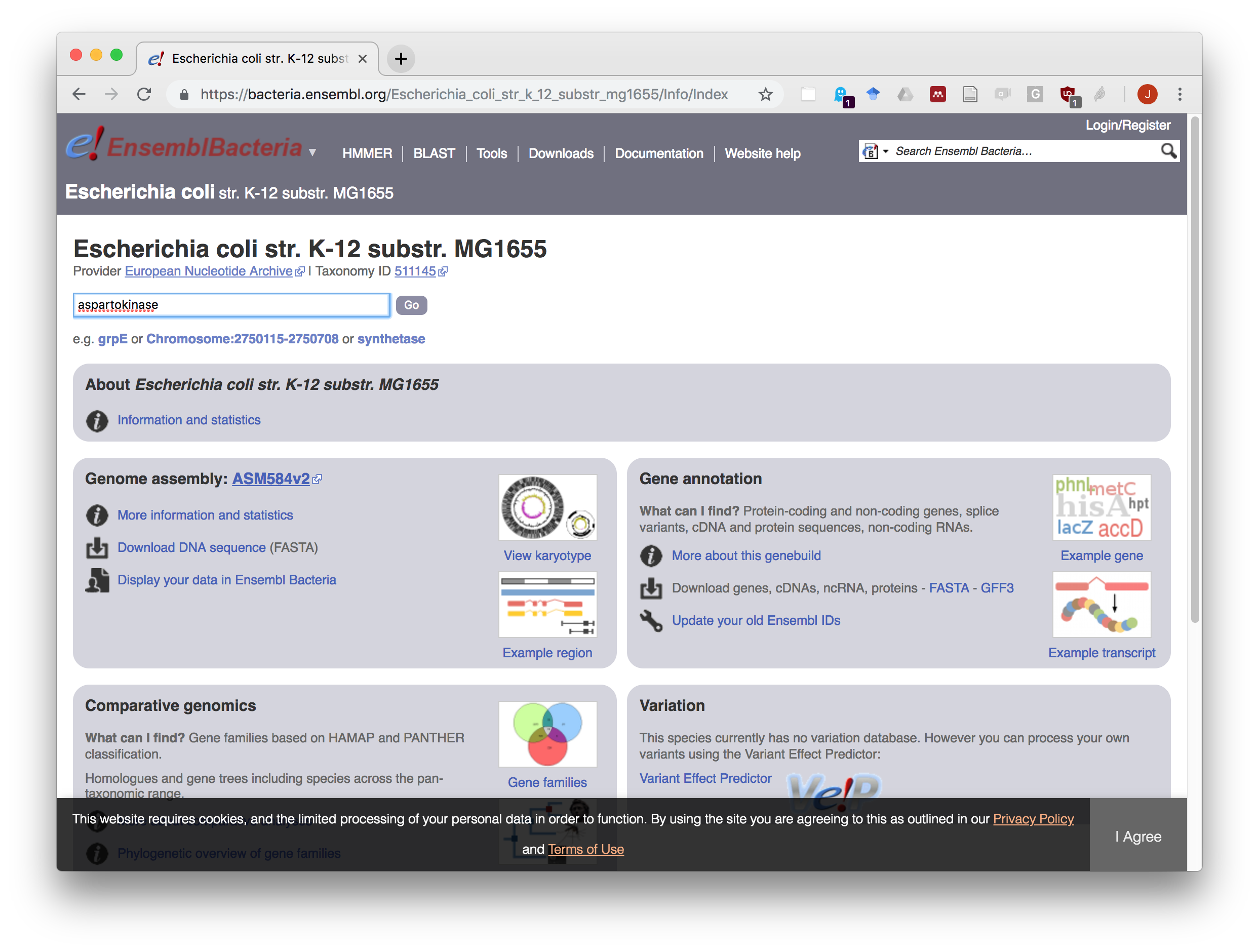
EnsemblGenomes gene search.
- Read the annotation of the three first matches. Note the names of the genes coding for these three enzymes.
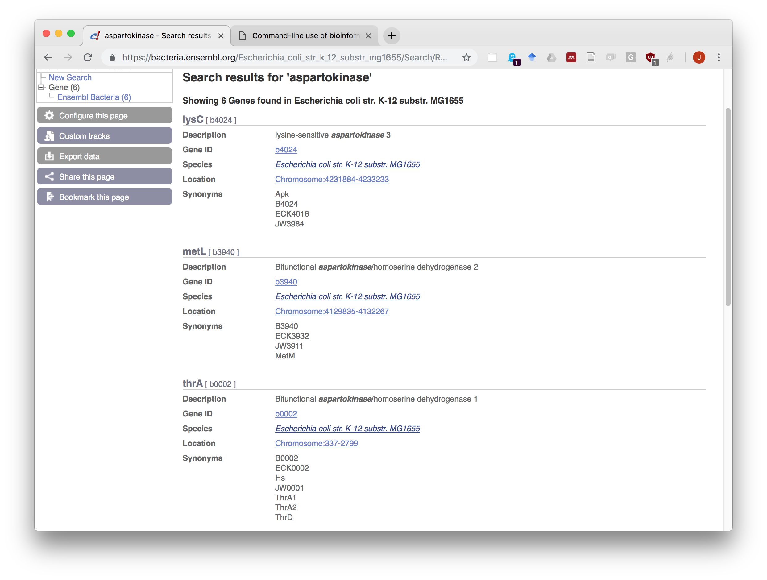
EnsemblGenomes search result for aspartokinase.
Downloading genomic features and protein sequences
We will use blast on the command line to search for homologs of E.coli aspartokinases in other bacterial genomes.
Each student will chose a different bacteria to perform the search.
Downloading protein sequences and gene annotations from Ensembl genome
In a separate window, open a connection to EnsemblGenomes Bacteria (https://bacteria.ensembl.org/).
Click on the **Downloads* link (you can also access it directly here: https://bacteria.ensembl.org/info/website/ftp/).
In the filter box, type MG1655. This select the subset of genomes whose name contains this string.

EnsemblGenomes download filter.
Click on the FASTA link in the column Protein sequences/
and select Copy link address.

EnsemblGenomes Link to download all protein sequences for a selected organism.
Come back to the Unix terminal of the IFB NNCR.
Create a directory for the current practical.
mkdir -p ~/bacteria_blast
cd ~/bacteria_blast- type
wget --no-clubberand paste the content of the clipboard. This should give the following command (note: at the tiem you run this tutorial, the release may be different, this one is from October 2018).
wget --no-clobber ftp://ftp.ensemblgenomes.org/pub/release-41/bacteria//fasta/bacteria_0_collection/escherichia_coli_str_k_12_substr_mg1655/pep/Escherichia_coli_str_k_12_substr_mg1655.ASM584v2.pep.all.fa.gzIf you want to know the meaning of the --no-clobber option you can checek wget manual with the command.
man wgetWe will now check if the file has been correctly downloaded, and uncompress it.
## Check that the file is there
ls -l

## Uncompress the file
gunzip Escherichia_coli_str_k_12_substr_mg1655.ASM584v2.pep.all.fa.gz

# Measure the size of the uncompressed file
du -k Escherichia_coli_str_k_12_substr_mg1655.ASM584v2.pep.all.fa

# Check the 20 fist lines of the file
head -n 20 Escherichia_coli_str_k_12_substr_mg1655.ASM584v2.pep.all.fa

# Check the 20 last lines of the file
tail -n 20 Escherichia_coli_str_k_12_substr_mg1655.ASM584v2.pep.all.fa
Downloading genome annotations
After having downloaded the protein sequences, we will download gene annotations. In EnsemblGenomes, annotations are available in different formats, including GTF, a text file with columns separated by tabulations.
We In the browser, come back to the EnsemblGenomes Bacteria Download site, select MG1655 and follow the same instructions as above to download and uncompress the GTF file.
Uncompress the gzip archive.
Solution
## Download genome annotation file (GTF format)
wget --no-clobber ftp://ftp.ensemblgenomes.org/pub/release-41/bacteria//gtf/bacteria_0_collection/escherichia_coli_str_k_12_substr_mg1655/Escherichia_coli_str_k_12_substr_mg1655.ASM584v2.41.gtf.gz

## Uncompress genome annotation file
gunzip Escherichia_coli_str_k_12_substr_mg1655.ASM584v2.41.gtf.gz

## Check that the uncompressed file is there
ls Escherichia_coli_str_k_12_substr_mg1655.ASM584v2.41.gtf

## Check the head of the annotaiton file
head -n 20 Escherichia_coli_str_k_12_substr_mg1655.ASM584v2.41.gtf

## Check the tail
tail -n 10 Escherichia_coli_str_k_12_substr_mg1655.ASM584v2.41.gtf
Exercise: genome annotations
As an exercise, you will now elaborate Unix commands to explore the content of E.coli genome annotations.
For this, we recommmend to use and combine the following commands. In order to fine-tune the parameters, read their manual on the Unix terminal by typing man [command_name] (for example man wc).
| Command | Usage |
|---|---|
| wc | count lines, words and characters of a file |
| cut | cut specific columns of a text file |
| grep | select rows of a file that match a given query (string, regular expression) |
| awk | a powerful tool to work on text files, combining row filters, column selections, and many other features. |
| sort | sort the rows of a text file based on user-specified columns. The sorting can be done either alphabetically or numerically, in ascending or descending order |
| uniq | discard redundant lines from a text file. The option -c counts the number of occurrences of each line in a redundant file |
You can learn more Unix commands by typing “Linux cheat sheet” in any Web search engine.
We ask you to write all the answers in a text file, with comments, in order to enable other people to reproduce all your commands.
Questions
- How many rows contains the GTF file for E.coli K12 MG1655 ?
How many annotation rows are there in the GTF file (for this, you need to discard the comment rows starting with a
#character) ?How many of these rows correspond to genes ?
Count the number of instnces of each feature type in the GTF file.
Select all the rows of the GTF file corresponding to a gene, and store them in a separate file named
genes_Escherichia_coli_str_k_12_substr_mg1655.ASM584v2.41.gtf.
Solution
Searching sequence similarities with BLAST
Activating the conda environment for blast on the NNCR cluster
In addition to facilitating the installation of software tools on different operating system, conda also permits to create modules that regroup a set of tools usually used together (for example NGS analysis, protein structure, proteomics, …).
The IFB NNCR cluster is already equipped with a series of conda environments with the classical bioinformatics tools. Before being able to use a tool, you must activate the corresponding environment.
## List the conda environments available on the system
$CONDA_HOME/bin/conda env list

## FInd the blast environment
$CONDA_HOME/bin/conda env list | grep -i blast

## Activate the blast environment.
source $CONDA_HOME/bin/activate blast-2.7.1

## Check the location of the blastp command
which blastp

## Deactivate the current environment.
source $CONDA_HOME/bin/deactivate
## Note the change in the shell prompt

## Re-activate the blast environment
source $CONDA_HOME/bin/activate blast-2.7.1
## Note the change in the shell prompt
Note: if you are working on a machine that does not belong to the federation of NNCR clusters, you can create the blast environment in your own conda folder with the following command (assuming that the conda package has been installed and that its executable files are in your path).
## ATTENTION: DO NOT RUN THIS COMMAND IF YOU ARE ON THE NNCR CLUSTER,
## because this would occupy a big space to reinstall BLAST in your
## own account, although it is already available for all users.

## Install blast
conda create -n blast-2.7.1 blast==2.7.1

## Install emboss
conda create -n emboss-6.6.0 emboss==6.6.0
Formatting the blast database for the reference genome
## Check the path of the program makeblastdb (it should be in your conda folder)
which makeblastdb

## Get the usage of makeblastdb (formal specification of the command syntax)
makeblastdb -h

## Get the help for makeblastdb (explanation of the options)
makeblastdb -help

## Build a BLAST database with all the protein sequences of E.coli
makeblastdb -in Escherichia_coli_str_k_12_substr_mg1655.ASM584v2.pep.all.fa  -dbtype prot

## Check the new files that were created with this commands.
## For this we list the files in reverse (-r) temporal (-t) order.
ls -1tr
The program makeblastdb created three files besides the input fasta file.
Escherichia_coli_str_k_12_substr_mg1655.ASM584v2.pep.all.fa.pin
Escherichia_coli_str_k_12_substr_mg1655.ASM584v2.pep.all.fa.phr
Escherichia_coli_str_k_12_substr_mg1655.ASM584v2.pep.all.fa.psq
These files contain an index of all the oligopeptites found in all the sequences of the fasta file. This “k-mer” index will be used by BLAST to rapidly find all the sequences in the database that match a query sequence, and use these short correspondences to start an alignment.
Read blastp manual
Since we want to search a protein database with protein query sequences, we will use the blastp command.
## Command  syntax
blastp -h

## Help
blastp -help
OK, the first contact is a bit frightening, because blastp has many options. This is because this program allows you to run queries in different modes, with different parameters, and to export the results in different formats.
In this tutorial we will show you the most usual ways to use the tool, and you will then be able to refine your search by combing back to the manual and understanding the use of additional options.
Downloading a query protein
We will first search similarities from a given protein of interest. We will start from the “askartokinase 3” protein from Escherichia coli, which is the product of the gene lysC.
Before starting the analysis, read the Uniprot record (https://www.uniprot.org/uniprot/P08660) in order to know the function and regulation of this protein.
We will use BLAST to identify all the proteins of Escherichia coli that have significant similarities with the aspartokinase 3.
For this we first need to download the sequence of this protein on our computer. The sequence can be downloaded directly from Uniprot.
wget --no-clobber https://www.uniprot.org/uniprot/P08660.fastaSimiliraty search for one sequence against a database
The following command search similarities for one or several query sequences provided in a fasta file (P08660.fasta) in a protein sequence database (Escherichia_coli_str_k_12_substr_mg1655.ASM584v2.pep.all.fa). By default, blastp prints the result on the screen, but we prefer to redirect it to a file in order to keep a trace of the result and inspect it later.
## Search similarities for aspartokinase 3 in E.coli proteome
blastp \
  -db Escherichia_coli_str_k_12_substr_mg1655.ASM584v2.pep.all.fa  \
  -query P08660.fasta \
  > lysC_vs_Ecoli.txt

## Check the result
less lysC_vs_Ecoli.txt
Question set 1
1. How many hits were found in total? 2. How many of these have an E-value higher than 1? 3. What was the threshold on the E-value for this blastp search? 4. With this threshold, how many hits would we expeect if we use a random sequence as query? 5. How many alignments would you consider significant in this result? 6. How many of these would you qualify of homologs? 7. For each of these putative homologs, is it a paralog, ortholog or “other log”? 8. Do you see a relationship between the E-value and some properties of the alignments?
Getting a tabular synthesis of blast results
By default, BLAST displays the detailed results of a similaty search, starting with a summary of the matches, followed by all the alignemnts. It can be convenient to generate a synthetic result indicating only the relevant statistics for each alignment. This can be done by tuning BLAST options.
Read blastp manual and find a way to tune the formatting options in order to get a tabular output with comments.
Solution
## Search similarities for aspartokinase 3 in E.coli proteome.
## Return the result as a synthetic table with the matching statistics for each hit.
blastp -outfmt 7 \
  -db Escherichia_coli_str_k_12_substr_mg1655.ASM584v2.pep.all.fa  \
  -query P08660.fasta \
  > lysC_vs_Ecoli_synthesis.tsv

## Check the result
more lysC_vs_Ecoli_synthesis.tsv
Negative control: blast against a shuffled sequence
In this section, we will perform a quick empirical test, by submitting a random sequence to blastp. For this, we will shuffle the aminoacids of the original query sequence.
Shuffling sequences with EMBOSS shuffleseq
## Activate the conda environment with the emboss software suite
source  $CONDA_HOME/bin/activate emboss-6.6.0

## Check that shuffleseq is available
which shuffleseq

## Get the suffle manual
shuffleseq -h

## Shuffle the apartokinase 3 sequence
shuffleseq -sequence P08660.fasta -outseq shuffled_lysC.fa

## Check the result
cat shuffled_lysC.fa

## Compare the shuffled seq with the original one
cat P08660.fasta
Here is an example of result (I just simplified the header of the shuffle output fasta sequence for the sake of readability).
Of course, your result should differ since each shuffling produces a randomized sequence.
>shuffled_lysC
VEAINNAVKRELSALGDVADLFVLEFDNDRLGWADAIIRVLLNTEMNGELKPAEVASAIV
GLIDEPELDTLVYSPLAGIFFLMCLIDFRGLGRREPTVPHSIMAGSGNALCRYFVTGLLL
LDTNAFAIRETKNLEAFVAEFQAADNFAQARNPANLPKLILCLSVNGVLQASPFFNLNEG
ADVVSESSAASLKADEDQSVITLEEDIVVTEGASSFDLALGLLMHLNVDRKVGAEWLEDE
VSPVMVEVLTLVLTQEALTVTSIALLRGDTRKRVGLVLNSFTSHDLIAPSLILIGTSLVT
RHFLVGAKVRIQERKASTSFRRLLAGRTETYRGLEIYAPCISMTTAVRRMQAGGIAHREI
QETIACRKSTELLSTIASPHAEVGFEAANGTLLGVLTADHVSMALQAVNGGESLPDEHRR
TVGDILTERVARLLLPFKEGPARTSSTLA
Exercise
Shuffle the aspartokinase 3 sequence with the tool
shuffleseq(found in the conda environmentemboss).Run a
blastpsearch with this shuffled sequence against all proteins of Escherichia coli.
Solution
## Run blast with the shuffled lysC sequence against all E.coli proteins
blastp \
  -db Escherichia_coli_str_k_12_substr_mg1655.ASM584v2.pep.all.fa  \
  -query shuffled_lysC.fa \
  > shuffled_lysC_vs_Ecoli.txt
## Check the result
less shuffled_lysC_vs_Ecoli.txt

## Run the same query with a tabular output
blastp -outfmt 7 \
  -db Escherichia_coli_str_k_12_substr_mg1655.ASM584v2.pep.all.fa  \
  -query shuffled_lysC.fa \
  > shuffled_lysC_vs_Ecoli_synthesis.tsv

## Check the result
less shuffled_lysC_vs_Ecoli_synthesis.tsv
Questions
- How many alignments would you expect by chance with the default blastp parameters?
- How many alignemnts did you get with the shuffled sequence?
- How many of these had an E-value smaller than 1?
- How many of these had an E-value smaller than 0.01?
- How many of these would you qualify of homologs?
Comparing all the proteins of a genome against another genome
Downloading a query genome
Open a connection to the EnsemblGenomes Download page https://bacteria.ensembl.org/info/website/ftp/
Identify the genome of your organism of interest (for this tutorial, I will choose Bacillus subtilis subsp. subtilis str. 168, but each student should take a different organism).
Download the genome annotation (GTF file) and protein sequences (fasta file).
Solution
## Download genome annotations for organism of interest
wget --no-clobber ftp://ftp.ensemblgenomes.org/pub/release-41/bacteria//gtf/bacteria_0_collection/bacillus_subtilis_subsp_subtilis_str_168/Bacillus_subtilis_subsp_subtilis_str_168.ASM904v1.41.gtf.gz

## Uncompress genome annotations for the organism of interest
gunzip -f Bacillus_subtilis_subsp_subtilis_str_168.ASM904v1.41.gtf.gz

## Download protein sequeces for query organism
wget --no-clobber ftp://ftp.ensemblgenomes.org/pub/release-41/bacteria//fasta/bacteria_0_collection/bacillus_subtilis_subsp_subtilis_str_168/pep/Bacillus_subtilis_subsp_subtilis_str_168.ASM904v1.pep.all.fa.gz

## Uncompress protein sequences for the organism of interest
gunzip -f Bacillus_subtilis_subsp_subtilis_str_168.ASM904v1.pep.all.fa.gz

## Check the result files
ls -l Bacillus_subtilis_subsp_subtilis_str_168.ASM904v1*


## Format the blas database for the organism of interest
makeblastdb -in Bacillus_subtilis_subsp_subtilis_str_168.ASM904v1.pep.all.fa -dbtype  prot
Identifying aspartokinase homologs in the proteome of interest
To identify homologs for a given protein, we can run a simple blastp search against the proteome of the organism of interest (in my case, Bacillus subtilis).
blastp \
  -db Bacillus_subtilis_subsp_subtilis_str_168.ASM904v1.pep.all.fa \
  -query P08660.fasta \
  > lysC_vs_Bacillus_subtilis.txt

blastp -outfmt 7\
  -db Bacillus_subtilis_subsp_subtilis_str_168.ASM904v1.pep.all.fa \
  -query P08660.fasta \
  > lysC_vs_Bacillus_subtilis_outfmt7.tsv
However this would return many false positives, since BLAST sets its default E-value to 10 (we thus expect ~10 false positives on average for such a search). To avoid this, blastp enables to control the expected number of false positives with a threshold on the E-value, using the option -evalue.
blastp  -evalue 0.00001 \
  -db Bacillus_subtilis_subsp_subtilis_str_168.ASM904v1.pep.all.fa \
  -query P08660.fasta \
  > lysC_vs_Bacillus_subtilis_eval0.00001.txt

## Check the alignments of aspartokinase homologs
less lysC_vs_Bacillus_subtilis_eval0.00001.txt

blastp -evalue 0.00001 -outfmt 7 \
  -db Bacillus_subtilis_subsp_subtilis_str_168.ASM904v1.pep.all.fa \
  -query P08660.fasta \
  > lysC_vs_Bacillus_subtilis_eval0.00001_outfmt7.tsv

## Check the matching statistics for the aspartokinase homologs
cat lysC_vs_Bacillus_subtilis_eval0.00001_outfmt7.tsv
Interpretation of the result
Note the strong reduction of the number of hits. By setting a stringent threshold of the e-value, we retained only the most significant hits. It is worth checking the other matching statistics, in particular the alignment length and the percentage of identical aminoacids: the threshold on e-value indirectly led to select the large alignments with a high percentage of identities (because these combined conditions are required to achieve a good statistical significance).
We can now check the function of the hits on the Uniprot database (http://uniprot.org).
Here is a link to the three proteins found in Bacillus subtlis:
https://www.uniprot.org/uniprot/?query=cab14807+OR+CAB12187+OR+CAB13549
What is the function of these proteins? In which pathways are these involved?
We can also try to understand the role of these aspartokinases by visualizing their place in metabolic pathwauys annotated in the BioCyc database.
https://biocyc.org/BSUB/NEW-IMAGE?type=PATHWAY&object=PWY-2941
All proteins of B.subtilis against all proteins of E. coli
Proteome-wise similarity search
Write a command that searches for similarities for all proteins of your proteome of interest against all proteins of E. coli, and prints the output in tab-delimited format with comment lines. Save the output in a file named
[your_organism]__vs__Escherichia_coli_blastp_outfmt7.tsv(relpace[your_organism]by the actual name of the organism you selected for this tutorial).Use
grepto select the non-comment lines and store them in a separate file named[your_organism]__vs__Escherichia_coli_blastp_table.tsv.
## Note : we prepend the command "time" to measure the computation time, just for the sake of curiosity
time blastp -outfmt 7 \
  -db Escherichia_coli_str_k_12_substr_mg1655.ASM584v2.pep.all.fa  \
  -query Bacillus_subtilis_subsp_subtilis_str_168.ASM904v1.pep.all.fa \
  > Bacillus_subtilis__vs__Escherichia_coli_blastp_outfmt7.tsv

## Create a separate file without comments
grep -v '^#' Bacillus_subtilis__vs__Escherichia_coli_blastp_outfmt7.tsv > Bacillus_subtilis__vs__Escherichia_coli_blastp_table.tsv

## Count the number of hits
wc -l Bacillus_subtilis__vs__Escherichia_coli_blastp_table.tsv
This search was realized with the default threshold on the E-value. The results is thus likely to includes a lot of false positives, since the default E-value for blastp is 10 ! For proteome-wise searches, one generally uses much more stringent threshold in order to only report highly significant matches.
Selecting significant hits
Run blast with a threshold of \(10^{-5}\) on the E-value and store the result in a separate file, in tabular format and without comments.
Note: we now discard the commands because this file will further be used to sort the hits by E-value.
## Note : we prepend the command "time" to measure the computation time, just for the sake of curiosity
time blastp -outfmt 6 -evalue 0.00001 \
  -db Escherichia_coli_str_k_12_substr_mg1655.ASM584v2.pep.all.fa  \
  -query Bacillus_subtilis_subsp_subtilis_str_168.ASM904v1.pep.all.fa \
  > Bacillus_subtilis__vs__Escherichia_coli_blastp_eval0.00001.tsv

## Count the number of hits
wc -l Bacillus_subtilis__vs__Escherichia_coli_blastp_eval0.00001.tsv
Counting the number of hits per protein
We can count the number of hits for each protein by combining a few unix commands: cut, sort and uniq. To this purpose, we will progressively build a single unix command line that chains these tools with the pipe symbol |, which sends the output of one unix command as input for the next one.
We will first cut the column containing the IDs of the proteins in the query proteome.
## Identify  the column containing the ID of the hits in the proteome of interest
head Bacillus_subtilis__vs__Escherichia_coli_blastp_eval0.00001.tsv

## Cut the first column (containing the ID of the hits in the query proteome)
cut -f 1 Bacillus_subtilis__vs__Escherichia_coli_blastp_eval0.00001.tsv | more

## Count the number of hits
cut -f 1 Bacillus_subtilis__vs__Escherichia_coli_blastp_eval0.00001.tsv | wc -l
We will now count the number of unique hits. For this we use the command sort with the argument -u (unique).
cut -f 1 Bacillus_subtilis__vs__Escherichia_coli_blastp_eval0.00001.tsv | sort -u | wc -lWe see that there are much less unique IDs than the total number of hits. However this does not yet tell us how many hits were found for each particular protein.
The program uniq suppresses redundant rows in a file. Combining sort and uniq has the same effect as using sort -u. Check by yourself.
cut -f 1 Bacillus_subtilis__vs__Escherichia_coli_blastp_eval0.00001.tsv | sort | uniq | wc -lIn addition, the program uniq contains an option -c enabling to report the number of occurrences of each row. Since we first used the cut command to obtain the column containing the protein IDs, each row analysed here corresponds to an ID of the query proteome. The command this counds the number of occurrences of each query protein in the blastp result file, which corresponds to its number of hits in the reference genome.
cut -f 1 Bacillus_subtilis__vs__Escherichia_coli_blastp_eval0.00001.tsv | sort | uniq -c | lessWe can now use the command sort (a second time in the same chain of commands) in order to sort the protein IDs by decreasing number of hits.
cut -f 1 Bacillus_subtilis__vs__Escherichia_coli_blastp_eval0.00001.tsv | sort | uniq -c |sort -nr -k 1 | lessFinally, we select the 10 first rows with the command head.
cut -f 1 Bacillus_subtilis__vs__Escherichia_coli_blastp_eval0.00001.tsv | sort | uniq -c |sort -nr -k 1 | head -n 10Interpretation of the results
Here is a link to the result for B.subtilis against E.coli
Read the annotations for some of these proteins with a very high number of hits, and try to identify their common characteristics. For example:
- Are they involved in particular pathways?
- Are they exerting particular molecular activities/functions?
- Are they located in particular cell compartments?
- Do they belong to particular protein families?
Based on this exploration of the annotations, do you understand why these proteins have so many hits?
Sorting hits by significance
We will now try to sort the hits by increasing E-value, in order to display the most significant hits n first place. For this, the simplest solution seems to use sort and specify a numeric sorting (option -n) on the numeric value of the \(11^{th}\) column (option -k 11), which contains the E-value. More precisely, we will specify -k 11,11 to sort on this column only, because the option -k 11 would use the \(11^{th}\) and all the subsequent columns as sorting keys. Let us look at the result.
## A first attempt to sort by E-value, not very convincint !
sort -k 11,11 -n Bacillus_subtilis__vs__Escherichia_coli_blastp_eval0.00001.tsv | less
Go down by a few pages by pressing the space bar, and pay a particular attention to the 11th column, which contains the E-value. Is the sorting correct ?
**Note: after hacing seen the result, type "q"** to quit `less`.The first rows contain hits with an E-value of 0. This does not properly speaking correspond to a null risk of false posiives, since there is a very small but non-null probability to observe a hit by chance, even if two proteins are very similar to each other. For blast, a \(0\) value in the \(11^{th}\) column indicates that the E-value is below the precision limit of computation, which is approximately \(1e-182\). E-values of 0 should thus be interpreted as “smaller than \(10^{-182}\)”.
At the transition between 0 E-values and non-zero E-values, you will notice that the sorting is incorrect. Here is the result we obtain with Bacillus subtilis.
...
CAB16047        AAC73707        56.673  517     ...   517     0.0     585
CAB16048        AAC75939        65.828  477     ...   479     0.0     676
CAB16138        AAC76764        52.564  624     ...   629     0.0     635
CAB11917        AAC76323        56.034  116     ...   116     1.00e-47        146
CAB12080        AAC76505        28.638  213     ...   229     1.00e-21        87.8
CAB12153        AAC73552        26.360  239     ...   564     1.00e-12        64.3
CAB12183        AAC73788        34.934  229     ...   223     1.00e-36        125
CAB12414        AAC74372        26.061  165     ...   195     1.00e-07        50.4
CAB12414        AAC76505        24.895  237     ...   223     1.00e-13        68.9
CAB12437        AAC74386        29.075  227     ...   220     1.00e-13        65.1
CAB12735        AAC76480        22.707  229     ...   242     1.00e-13        65.5
...
Why are the E-values not sorted correctly? Apparently, the Unix sort command does not support the scientific notation, and thus mis-handles numbers like 1.00e-36 or 1.00e-12.
To solve this, people use different tricks. Mine is to use awk in order to add a column with a significance score, which I define as the minus log of the E-value.
\[sig = -log_{10}(\text{Evalue})\]
I do a double transformation, to replace infinite values (resulting from null E-values, since \(-log_{10}(0) = \text{-inf}\)) by a number, which I arbitrarily set to \(200\) (higher than the 182).
Note: by default, the log() function computes natural logarithms. Base 10 logarithms can be computed easily by dividing the result by the natural logarithm of 10.
\[log_{10}(x) = log_e(x) / log_e(10)\]
## Sort BLAST hits on a column with significance, computed with awk
awk '{sig= -log($11) / log(10); print $0"\t" sig}' \
  Bacillus_subtilis__vs__Escherichia_coli_blastp_eval0.00001.tsv \
  | awk '{ sub("inf", "200"); print }' \
  | sort -k 13,13 -n -r \
  | less
Sorting hits by significance + bit score
Adapt the above command to sort on a double key:
- Primary key: decreasing significance (as computed above)
- Secondary key: decreasing bit score (the $12^{th}$ column of BLAST output)
Store the result in a file named [your_organism]__vs__Escherichia_coli_blastp_sorted.tsv
Solution
## Define an environment variable with the name of the sorted hits (this will be useful for further processing)
BLAST_HITS_SORTED=Bacillus_subtilis__vs__Escherichia_coli_blastp_sorted.tsv

## Sort BLAST hits by decreasing significance and decreasing bit score
awk '{sig= -log($11) / log(10); print $0"\t" sig}' \
  Bacillus_subtilis__vs__Escherichia_coli_blastp_eval0.00001.tsv \
  | awk '{ sub("inf", "200"); print }' \
  | sort -k 13,13 -k 12,12 -n -r \
  > ${BLAST_HITS_SORTED}

## Check the result
less ${BLAST_HITS_SORTED}
Computing blast hit ranks
Starting from the sorted blast hits, compute
- a rank of the hits according to the query protein (`qrank`),
- another rank according to the "subject" protein (`srank`), i.e. the protein found in the blast database of your reference organism. Definition: by Best hit we mean the most significant alignment, i.e. the alignment with the smallest E-value. In case of identical E-values, the bit score is used as secondary ranking criterion, as we did above.
Tip: awk enables to compute ranks by incrementing a counter at each occurrence of a given value (e.g. a protein identifier) in a given column (e.g. the first column, which contains query protein IDs).
The following command adds a column to the sorted blast hits, indicating the occurrence number of each value of the first column. Since our file is sorted by E-value, this corresponds to the rank of the hits according to the query sequences (we therefore name the variable qrank).
awk '{ qrank[$1]++ ; print $0"\t"qrank[$1]}' ${BLAST_HITS_SORTED} | lessWe can now complete this command by computing a second variable which indicates the rank of each hit according to the “subject”" sequence (srank), i.e. the sequence of the blast database.
BLAST_HITS_RANKED=Bacillus_subtilis__vs__Escherichia_coli_blastp_ranks.tsv
awk '{ qrank[$1]++ ; srank[$2]++ ; print $0"\t"qrank[$1]"\t"srank[$2]}' \
  ${BLAST_HITS_SORTED} > ${BLAST_HITS_RANKED}

## Check the result
less ${BLAST_HITS_RANKED}
less does more or less the same as more
With the less command, you can browse the content by pressing the space bar in order to see the next “page”. In the beginning of the file, most ranks are 1 in the two last columns, because the very low E-values generally correspond to the bidirectional best hit. As you go down, you will notice some hits with larger rank values for the srank and qrank columns, indicating that the query or subject sequences have multiple hits.
Finding best hits
With the ranked blast hits, use the awk command to select:
- the best hit for each protein of the query organism (query BH);
- the best hit for each protein of the reference organism (subject BH);
- the bidirectional best hit (BBH)
Save each result in a separate file, and count the number of hits in each file.
Solution
## Best hits per query sequence
BLAST_QUERY_BH=Bacillus_subtilis__vs__Escherichia_coli_blastp_query_BH.tsv
awk '$14 == 1' ${BLAST_HITS_RANKED} > ${BLAST_QUERY_BH}

## Best hits per subject sequence
BLAST_SUBJECT_BH=Bacillus_subtilis__vs__Escherichia_coli_blastp_subject_BH.tsv
awk '$15 == 1' ${BLAST_HITS_RANKED} > ${BLAST_SUBJECT_BH}

## Bidirectional best hits
BLAST_BBH=Bacillus_subtilis__vs__Escherichia_coli_blastp_BBH.tsv
awk '$14 == 1 && $15 == 1' ${BLAST_HITS_RANKED} > ${BLAST_BBH}

## Count number of best hits
wc -l  ${BLAST_QUERY_BH} ${BLAST_SUBJECT_BH} ${BLAST_BBH}
All proteins from E. coli versus E. coli
Exercise: build a command that compares the sequences of all the E.coli proteins against each other, and store the results in a tab-delimited file with a single line per hit (we do not need the alignments).
Devoir-maison
Informations
Ce devoir-maison peut être réalisé en combinant quelques commandes en ligne (
cut,grep,awk,sort,uniq,wc,diff) et l’outil bioinformatiqueblastp.Nous vous recommandons de lire les manuels de ces commandes, ou de consulter quelques tutoriels. En particulier, il sera utile de connaître la syntaxe de
awkpour manipuler des chaînes de caractères (substitution, impression de colonnes sélectionnées) et pour numéroter les lignes. On trouve par exemple des informations ici: http://www.catonmat.net/blog/awk-one-liners-explained-part-two/.Le rendu de ce TP inclut un script bash rédigé de façon à être compréhensible par un lecteur non averti (commentez le code, nommez les variables de façon indicative, …). Ce script devra également être paramétrisable pour analyser d’autres organismes que le vôtre. A cette fin, définissez dès le début des variables pour les organismes d’intérêt (
QUERY_ORG) et de référence (REF_ORG), ains que pour les noms de fichiers d’input et output. En principe l’enseignant devra pouvoir refaire tourner toutes vos analyses à partir de votre script.La seconde pièce du rendu sera un rapport d’interprétation synthétique.
Ci-dessous (et dans votre rapport) nous désignerons les hits avec une E-valeur inférieure à 1e-5 comme “homologues prédits” ou plus simplement “homologues”.
Modèle de rapport
Je fournis ci-dessous 2 modèles de rapport pour le devoir-maison du TP proteome BLAST.
- Format docx (peut s’ouvrir avec LibreOffice ou avec un éditeur de texte commercial).
Pour les geeks: un fichier R markdown (extension Rmd), que j’ai utilisé pour générer le modèle de rapport docs. Ce fichier Rmd peut être édité et compilé avec RStudio de façon relativement intuitive, pour produire un rapport HTML, pdf ou docx. Comme vous n’avez pas encore eu l’occasion d’apprendre R markdown, il n’y a aucune obligation à utiliser ce format, mais je vous le fournis déjà pour ceux qui seraient tentés de se lancer. Si c’est votre cas, soumettez à la fois le fichier Rmd et le résultat de votre compilation (html, word ou docx).
Questions
Faites tourner blast pour toutes les protéines de votre organisme d’intérêt contre toutes celles de E.coli, en sélectionnant un fichier de sortie tabulaire sans commentaires, et un seuil de \(10^{-5}\) sur la E-valeur. Triez les hits par signiticativité (clé primaire) et par bit score (clé secondaire), puis calculez les rangs des hits en fonction des séquences “query” et “subject” comme nous l’avons fait dans le tutoriel.
Comptez
- le nombre total de hits
- le nombre total de paires de protéines avec un hit
- le nombre de protéines de votre ortanisme d’intérêt ayant au moins un hit chez E.coli
- le nombre de protéines d’E.coli pour lesquelles au moins un hit a été trouvé à partir de votre organisme d’intérêt
- le nombre de best hits pour l’organisme d’intérêt
- le nombre de best hits pour l’organisme de référence (E.coli)
- le nombre de best hits bidirectionnels
Générez un fichier qui indique le nombre d’homologues prédits par protéine de l’organisme d’intérêt. Ce fichier contiendra une ligne par protéine, et deux colonnes, indiquant respectivement le nombre de hits et l’ID de la protéine (
uniq -c). Triez les résultats par nombre décroissant de hits (les protéines ayant le plus grand nombre de hits s’affichent en premier lieu). Afficher les 10 premières lignes du fichier.
Question d’interprétation : Utilisez Uniprot pour savoir quelle est la fonction biologique des protéines présentant un très grand nombre de hits. Cette fonction permet-elle de comprendre ce nombre excessif de hits ?
- Calculez le nombre de protéines de l’organisme d’intérêt sans homologue prédit.
Question d’interprétation : Comment interprétez-vous ces protéines sans hit ?
- Calculer la distribution du nombre d’homologues par protéine (combien de protéines ont 0, 1, 2, 3, … homologues).
Question d’interprétation : quel est le nombre moyen de hits ? Combien de protéines ont un seul hit ? Comment interpréteriez-vous ces deux nombres en termes évolutifs ?
- Identifiez dans les deux comparaisons (votre organisme vs E.coli et E.coli vs votre organisme) toutes les homologies concernant des aspartokinase. Sur base de la règle du bidirectional best hit, tentez d’établir les relations d’orthologie et de paralogie entre chaque paire de protéines, et représentez les résultats dans un tableau avec les gènes de votre organisme sur les lignes, les gènes de E.coli sur les colonnes, et en indiquant “P”, “O”, ou “I” pour paralogie, orthologie ou identité, respectivement.
Question d’interprétation : comment interprétez-vous ces résultats en terme de voies métaboliques ? N’hésitez pas à constuler des ressources complémentaires (KEGG, MetaCyc, …).
Question bonus pour les acharnés
Utilisez le programme
shuffleseqpour permuter les séquences de votre organisme d’intérêt, et effectuez les mêmes analyses avec ces séquences aléatoires. Comparez les résultats et ceux obtenus avec le protéome de votre organisme d’intérê.Comparez le protéome de E.coli à lui-même et calculez les nombres de hits.
Utilisez votre script pour effectuer les analyses dans l’autre sens, en inversant les noms d’organismes d’intérêt (QUERY_ORG) et de référence (REF_ORG).